3.1.1 Definition of the GREEN's Function
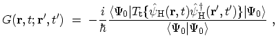
The time-ordered single-particle GREEN's function at zero temperature is
defined as [189]
 |
(3.2) |
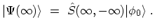
where
 is the ground-state of the interacting system in the
HEISENBERG picture (Appendix B) and
is the ground-state of the interacting system in the
HEISENBERG picture (Appendix B) and
 is the
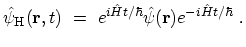
time-ordering operator defined in (B.21). The field operator
is the
time-ordering operator defined in (B.21). The field operator
 in the HEISENBERG picture is given by
 |
(3.3) |
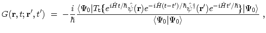
Inserting (3.3) into (3.2), the physical
interpretation of the GREEN's function becomes obvious
 |
(3.4) |
If  , the GREEN's function
 is the
probability amplitude that a particle created at time
is the
probability amplitude that a particle created at time  at place
 moves to time
  and place
  . This follows from the definition of
. At zero time the system is at the ground-state
. This follows from the definition of
. At zero time the system is at the ground-state
 . The system then evolves to time with the operator
 . At this time
 creates a
particle at place
. Then, the system continues its evolution from
to with the operator
creates a
particle at place
. Then, the system continues its evolution from
to with the operator
 , after which
 annihilates the particle at place . The
system returns to the initial ground-state with the operator
annihilates the particle at place . The
system returns to the initial ground-state with the operator
 . In a similar way, if
  , the field operator creates a hole
at time , and the system then propagates according to the HAMILTONian
, the field operator creates a hole
at time , and the system then propagates according to the HAMILTONian
 . These holes can be interpreted as particles traveling backward in
time [191]. The probability amplitude that a hole created at time
at place moves to time and place
is again just
the GREEN's function for
. These holes can be interpreted as particles traveling backward in
time [191]. The probability amplitude that a hole created at time
at place moves to time and place
is again just
the GREEN's function for  .
.
To calculate
, a perturbation expansion is very
useful. However, the definition of the GREEN's function
in (3.2) does not allow a direct solution, since it involves
the exact ground-states of the interacting HAMILTONian , which is one
of the things to be calculated. In the interaction representation the HAMILTON
ian is expressed in terms of the non-interacting and interacting parts, see the
equation (3.1). The ground state of the
non-interacting part,
 , can be calculated easily. Therefore, one
tries to express the ground state of the interacting system
in terms of the ground state of the non-interacting one
, can be calculated easily. Therefore, one
tries to express the ground state of the interacting system
in terms of the ground state of the non-interacting one
 . For
that purpose, in equation (B.18) one adds to the operator
. For
that purpose, in equation (B.18) one adds to the operator
 a factor
 , which
switches the interaction off at
, which
switches the interaction off at
 [189].
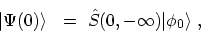
The non-interacting ground state
is assigned to the system
at
[189].
The non-interacting ground state
is assigned to the system
at
 and the connection to
is formed
by the GELL-MANN and Low theorem [192]
and the connection to
is formed
by the GELL-MANN and Low theorem [192]
 |
(3.5) |
where the  operator in defined in Appendix B.4.
The traditional argument is that one starts from
with a
wave function
operator in defined in Appendix B.4.
The traditional argument is that one starts from
with a
wave function  which does not contain the effects of the interaction
 . The operator
 brings this wave
function up to the present,
brings this wave
function up to the present,  [189]. Thus one has the wave
function which contains the effects of the interaction
,
so that it is an eigenstate of . As
[189]. Thus one has the wave
function which contains the effects of the interaction
,
so that it is an eigenstate of . As
 , one gets
 |
(3.6) |
One possible assumption is that
 must be related to
. The system returns to its ground state for
except for a phase factor [190]
must be related to
. The system returns to its ground state for
except for a phase factor [190]
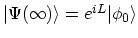 which implies that,
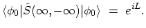 |
(3.7) |
An alternative to this assumption is discussed in Section 3.3.2.
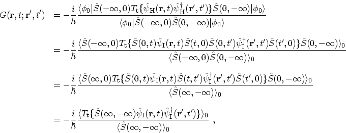
Using the relation (3.5) for the ground-state,
equation (3.2) becomes
 |
(3.8) |
where the short-hand notation
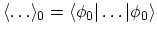 is introduced
to represent the expectation value over the ground-state of the non-interacting
system at zero temperature. The transition from the first to the second line
is achieved by using (B.13) for converting the
HEISENBERG representation of operators into the interaction
representation. The second step is obtained by taking account of the properties
of the operators described in Appendix B.4 and the
return of the system to its ground-state as
. In the forth
line the operator
is introduced
to represent the expectation value over the ground-state of the non-interacting
system at zero temperature. The transition from the first to the second line
is achieved by using (B.13) for converting the
HEISENBERG representation of operators into the interaction
representation. The second step is obtained by taking account of the properties
of the operators described in Appendix B.4 and the
return of the system to its ground-state as
. In the forth
line the operator
 contains several time intervals
 ,
,  , and
, and
 . The
operator
automatically sorts these intervals so that they act in their proper sequences.
Replacing operator with its formal definition (see (B.24)) one
gets
. The
operator
automatically sorts these intervals so that they act in their proper sequences.
Replacing operator with its formal definition (see (B.24)) one
gets
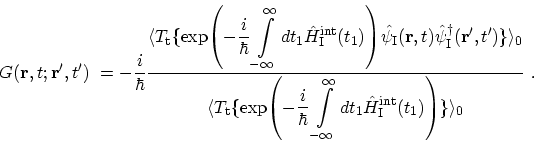 |
(3.9) |
M. Pourfath: Numerical Study of Quantum Transport in Carbon Nanotube-Based Transistors