


| | |
So far differential structures have been explored which have proved essential in the development of physical sciences. Differential descriptions are, however, not the only descriptions available. In the following the concepts for the dual operation of differentiation are outlined, which not only provide different descriptions as in Section 5.6, but also inspire different methodologies. It requires a few very basic definitions on which to build.
Definition 87 (Borel set) A set which is obtained from open sets of a topological space (Definition 29) using a countable number of unions, intersections and complements is called a Borel set.
Another term is introduced in order to simplify the subsequent Definition 89.
Definition 88 ( -algebra) A non-empty collection
  of subsets of a set
  such that it
is closed under countably many unions, intersections, or complements of elements is called a
such that it
is closed under countably many unions, intersections, or complements of elements is called a
 -algebra.
In the case of dealing with topological spaces a particular  -algebra, which contains all open sets, is of
special interest.
-algebra, which contains all open sets, is of
special interest.
Definition 89 (Borel- -algebra) The set of all Borel sets (Definition 87) is the
Borel-
-algebra) The set of all Borel sets (Definition 87) is the
Borel- -algebra.
Definition 90 (Measurable space) The pair  of a set
  along with a
  -algebra
  is called a measurable space.
Definition 91 (Signed measure) A mapping

 -algebra
  (Definition 88) over the set
  ,
such that for any collection of disjoint sets
,
such that for any collection of disjoint sets  in
in  it holds that

When the mapping  is restricted to values
  , it is called simply a measure.
Definition 92 (Measure space) A measurable space  (Definition 90) along with a
measure
(Definition 90) along with a
measure  forming the triple of a set
  , a
, a  -algebra (Definition 88) and a measure
 form a measure space.
Providing a measure on a Borel- -algebra (Definition 89) is an essential step of defining integration
on topological spaces (Definition 29) such as manifolds (Definition 35).
-algebra (Definition 89) is an essential step of defining integration
on topological spaces (Definition 29) such as manifolds (Definition 35).
The Lebesgue measure is a particular choice for a measure which is related to an interval of  in the
form
in the
form
![I = [a,b] ∈ ℝ λ (I) = b − a. (4.167)](whole638x.png)
 is then simply obtained by
![n n ∏n
I = [a1,b1] × ...× [an,bn] ∈ ℝ λ(I) = (bi − ai) (4.168)
i=1](whole640x.png)
Definition 93 (Almost everywhere) A property is said to apply almost everywhere in a
measure space  , if the complement of the set, where the property does not hold, has
measure
, if the complement of the set, where the property does not hold, has
measure  .
.
Using a measure it is possible to introduce the notion of integration of functions. The first step is to examine functions of the form

 , also called step functions. An integral of
  using a measure
  is then obtained by

Definition 94 (Integral of a function) Using the step functions, the integral of functions of the form


It follows from this definition that the integral does not change its value as long as only function values
associated with sets of measure  are changed.
The integral obtained by using a Lebesgue measure is called the Lebesgue integral, which while not being the most general notion of integration available, shall be sufficient for matters at hand.
In the context of manifolds the Borel- -algebra (Definition 89) can be presented very powerfully by
the concept of chains [78], which provide convenient methods of expression for operations on the
integration domain.
-algebra (Definition 89) can be presented very powerfully by
the concept of chains [78], which provide convenient methods of expression for operations on the
integration domain.
It should be noted that the integration domain and the domain of the function being integrated must agree for the integral to be well defined (Definition 94). An example of such agreement, which may still be embedded in a greater structure of a manifold (Definition 35) is given next.
Definition 95 (Curve integrals) The integral of a  -form (Definition 50) along a segment of a
curve
-form (Definition 50) along a segment of a
curve  (Definition 46) connecting two points
  and
and  is simply defined
as
is simply defined
as
![∫ ∫
ω = ω(φ˙(t))dt. (4.173)
φ [a,b]](whole656x.png)
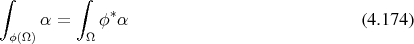
One of the most important properties of integration is that operations on the integration domain may be mapped to the integrand by pullback (Definition 44).
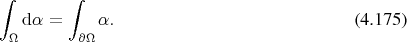
 being the boundary operation
  called
Stokes’ theorem, which asserts that when integrating a
called
Stokes’ theorem, which asserts that when integrating a  -form on a
  -integration domain it follows
that
-integration domain it follows
that
| | |