Hamiltonian Formalism

5.3 Hamiltonian Formalism

While the Lagrangian formalism already provides extensive capabilities to handle elaborate problems, further reﬁnement is possible resulting in the so called phase space, which also makes concepts available, which can even be carried beyond the conﬁnes of classical mechanics.

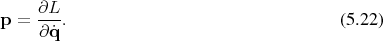
Motivated by the aim to ﬁnd a simpler, more symmetric expression of the equation of motion as given in Equation 5.14, it is fruitful to utilize the fact from the settings of the Lagrangian in Equation 5.10 and Equation 5.12, from which follows that the momentum is expressible as

∂L p = -∂˙q . (5.22)

Adopting this momentum to express the degrees of freedom previously expressed by $q˙$ using a Legendre map (Deﬁnition 53) results in

H (q,p, t) = ⟨p, ˙q⟩ − L(q,q˙, t), (5 .23)

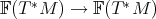
thus deﬁning a Hamiltonian corresponding to a given Lagrangian. Contrary to the Lagrangian, which is a function on the tangent bundle $T M$ , the Hamiltonian is a function on the co-tangent bundle $∗ T M$ , which is called the phase space.

H (q,p ) : T∗M → ℝ (5.24)

This is the deﬁning expression in the Hamiltonian formalism. Furthermore, the cotangent bundle is equipped with a symplectic structure (see Deﬁnition 81), which turns the cotangent bundle $T∗M$ of an $n$ dimensional base manifold into a symplectic manifold (Deﬁnition 82) of dimension $2n$ . Among the great strengths of the Hamilton formalism is the fact that Hamilton’s equations can be expressed using this geometric structure inherent to the phase space.

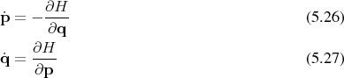
The symplectic nature of the manifold used ensures that it is always possible, as asserted by Deﬁnition 84, to ﬁnd coordinates such that

[p,p ] = 0, (5 .25a) [ [q,q ]] = 0, (5.25b) pi,qj = δji, (5 .25c)

called canonical coordinates.

The equations of motion as observed in the Lagrangian case take on the simpler, almost symmetric form

∂H ˙p = − ---- (5.26) ∂q ∂H-- ˙q = ∂p (5.27)

called Hamilton’s equations. Together they deﬁne a vector ﬁeld $vH$ (Deﬁnition 62) along with associated integral curves $γH (t)$ (Deﬁnition 63), which all taken together deﬁne the phase ﬂow $Φt$ (Deﬁnition 67). This phase ﬂow is a symplectomorphism (Deﬁnition 83), thus leaving the symplectic structure (Deﬁnition 81) of the manifold invariant.

The vector ﬁeld due to the Hamiltonian $H$ can be expressed utilizing the geometrical structure (compare Equation 4.162) inherent to the phase space.

vH = IdH = γ˙H (5.28)

This vector ﬁeld provides the opportunity to express the evolution of the system under investigation as the parameter $t$ changes. In case of a function $f$ , which measures a quantity of interest in the phase space

f(q,p ) ∈ 𝔽 (T∗M ) : T ∗M → ℝ, (5 .29)

the evolution with regard to the parameter $t$ due to the Hamiltonian and its own dependence on the parameter is then simply given by

˙f = vH (f) + ∂f-, (5 .30) ∂t

recalling that a vector ﬁeld is a mapping of the form $𝔽(T∗M ) → 𝔽 (T ∗M )$ (see Equation 4.109), which is usually given explicitly using the Poisson bracket (Deﬁnition 86) in the form

f˙= df-= {f,H } + ∂f-, (5 .31) dt ∂t

which indicates how the geometry of the system, deﬁned by the Hamiltonian, is responsible for its evolution.