Scallop Geometry

5.2.1 Scallop Geometry

An accurate evaluation of the hypothesis relies on a good description of the scallop’s geometric shape. A parabolic-like shape is suggested, as depicted on the previous cross sectional TSV images in Fig. 5.2. The height and width of each scallop is estimated to be 2 $μ$ m and 0.5 $μ$ m respectively.

The scallops’ geometry can be obtained using level set based Bosch process simulations. However, to understand their influence on the TSV, different combinations of height and width were studied. In order to study various scallop shapes, level set simulations are an unfeasible approach, because the simulations can take a considerable amount of time and the simulation results are not easily adaptable to the finite element tools used in this work. Thus, an alternative solution was applied. A single Bosch simulation was carried out, as shown in Fig. 5.4, and based on it an entire set of structures was manually constructed for several dimensional combinations. The scallop shape is then fitted to rational quadratic Bézier curves [88], for which the general form is given by

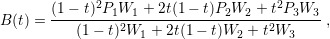(1 − t)2P1W1 + 2t(1 − t)P2W2 + t2P3W3 B (t) = ----------2-------------------2------ , (1 − t)W1 + 2t(1− t)W2 + t W3

(5.1)

where P1, P2, and P3 are control points as depicted in Fig. 5.5. W1, W2, and W3 are weights used for curvature control corresponding to each point of the curve (P1, P2, and P3, respectively), and t is the curvature parameter which varies between 0 and 1. Fig. 5.4 depicts a visual comparison between the Bézier curve description of the scallop, the Bosch simulation, and the observed scallop along a processed TSV sidewall.

pict

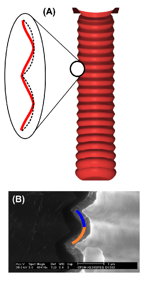
Figure 5.4.:

Comparison between the Bézier curve description of the scallops to the Bosch process simulation (a) and the fabricated scallop (b). Bézier curves create sharp points between the scallops, which could lead to unrealistic stress build-up at these meeting points during simulation.

Two Bézier curves were used to form a scallop, as depicted in Fig. 5.5. For each scallop, the curvature, size, and width were controlled by an appropriate choice of weights and points in relation to both curves, following the rules below:

pict

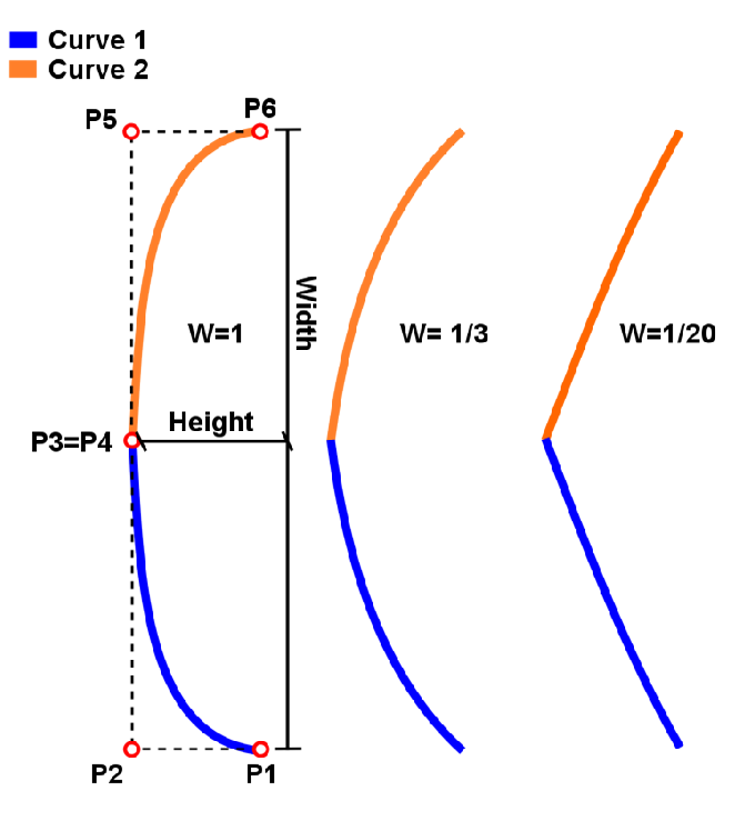
Figure 5.5.:

Scallop shape approximation by two Bézier curves. The curvature, height, and width are controlled by the weights.

P1 and P6 must be on the intended TSV wall (without scallops) and the distance between them defines a scallop’s width.
The distance between P1 and P2 defines the maximum scallop’s height which is reached at the middle of the scallop’s width.
P1 and P2 are placed on the same side of the scallop while P5 and P6 are placed on the opposite side of the scallop.
The weights W1, W3, W4, and W6 are given the value 1. The weights W2 and W5 have the same value (which controls the scallop’s curvature), W2=W5=W. It was chosen W=1/3.

Although this approach describes the scallops’ parabolic shape, the junction between them is smoother than the Bézier curve can represent. This could lead to singularities during simulation, resulting in high stress at the points where two scallops meet.

[next] [prev] [prev-tail] [front] [up]