During decades of hot-carrier degradation investigations, different modeling
approaches have been proposed. Most models concentrate on the degradation of
the
![]() interface where the creation of interface states due to bond
breaking has to be captured. Many of these approaches are phenomenological and
use empirical expressions to describe the degradation. Therefore, they
commonly only work for a special group of devices and have limited validity.
Their predictive character is commonly low, and scaling of devices often
requires parameter re-calibration. As a result, the need for models reproducing
the physical phenomena responsible for hot-carrier degradation has grown.
Therefore, it is of great importance to reveal and capture the physical picture
behind HCD and be able to predict the degradation of arbitrary devices.
interface where the creation of interface states due to bond
breaking has to be captured. Many of these approaches are phenomenological and
use empirical expressions to describe the degradation. Therefore, they
commonly only work for a special group of devices and have limited validity.
Their predictive character is commonly low, and scaling of devices often
requires parameter re-calibration. As a result, the need for models reproducing
the physical phenomena responsible for hot-carrier degradation has grown.
Therefore, it is of great importance to reveal and capture the physical picture
behind HCD and be able to predict the degradation of arbitrary devices.
The electric field has long been used as the main driving force for the degradation process. But it soon became clear that the electric field alone is often not enough for proper modeling and the carrier energy distribution needs to be considered. One of the most important physical modeling approaches considering the carrier energies can be found in the work of Hess [236], Rauch and La Rosa [212], and Bravaix [223].
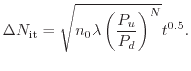
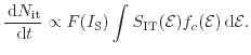
Hu et al. [203] proposed a model for interface trap generation, assuming that
bond dissociation is triggered by hot-carriers having energies above a certain
threshold energy level
![]() (assumed to be 3.7 eV in
[203]). Deduced from the lucky electron concept [192], a
relation for the interface trap generation can be written similarly to the
lucky electron model used for impact-ionization in (5.17) as
(assumed to be 3.7 eV in
[203]). Deduced from the lucky electron concept [192], a
relation for the interface trap generation can be written similarly to the
lucky electron model used for impact-ionization in (5.17) as
![$\displaystyle \ensuremath{\Delta N_\mathrm{it}}= C \left[ t \frac{\ensuremath{I...
...th{\mathcal{E}}_\mathrm{IT}/\ensuremath{\mathcal{E}}_\mathrm{II}} \right] ^ n .$](img462.png) |
(6.2) |
This simple and often used model from the year 1985 cannot reproduce the degradation in modern devices. In extremely down-scaled devices the limitations of the model become clear: due to the small extensions the non-locality of the electric field leads to overestimated degradations. On the other hand, in low-voltage operation the energies stay below the threshold energy leading to vanishing degradation. Although the model shows to deliver wrong results for advanced and especially for highly down-scaled devices, it is still used for extrapolations of the device life-time and might still be the most widely used model. There are also extensions of the lucky electron model presented by different authors. Among them are Takeda and Suzuki [237], Goo [238], and Dreesen [239].
The work of Hess et al. [230,235,236] incorporates the two
degradation mechanisms, the SP and MP processes, within the same
framework. Breaking a bond means the release of bound hydrogen and the related
desorption rate is derived considering the two degradation mechanisms:
![]() Since these processes are not fully independent, this
separation is only assumed to be an approximation.
Since these processes are not fully independent, this
separation is only assumed to be an approximation.
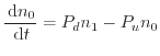
The SP process describes the excitation of one of the bonding electrons to an anti-bonding state by a solitary hot carrier. Such an excitation leads to dissociation of the bond followed by release of the hydrogen atom. The dissociation rate can be estimated using
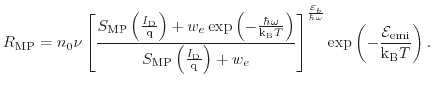
The MP desorption rate is described in this model using the truncated harmonic
oscillator (see Fig. 6.2) which can also be used to
explain the giant isotope effect [234]. The bond energetics is
described by a ladder of ![]() bonded levels. The MP process initiates an
excitation of the bond and an increase of the energy climbing the ladder of the
energetic states. The vibrational mode excitation ends when the hydrogen is
situated on the last bonded state. If the next portion of energy deposited by
channel carriers exceeds the emission energy
bonded levels. The MP process initiates an
excitation of the bond and an increase of the energy climbing the ladder of the
energetic states. The vibrational mode excitation ends when the hydrogen is
situated on the last bonded state. If the next portion of energy deposited by
channel carriers exceeds the emission energy
![]() the
hydrogen is released to the transport state. In the reverse direction the
passivation rate is determined by the barrier energy
the
hydrogen is released to the transport state. In the reverse direction the
passivation rate is determined by the barrier energy
![]()
![\includegraphics[height=45mm]{figures/harmonic_oscillator_html}](img475.png) |
Finally the desorption rate for de-passivation due to the MP process is written as [230]
![$\displaystyle R_\ensuremath{\mathrm{MP}}\propto \left\{ \left( \frac{\ensuremat...
...ht] ^ {-\frac{\ensuremath{\mathcal{E}}\mathrm{b}}{\ensuremath{\hbar \omega}}} ,$](img476.png) |
(6.5) |
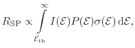
![$\displaystyle P_u \propto \int_0 ^{\infty} I(\ensuremath{\mathcal{E}}) \sigma_\...
...emath{\hbar \omega}) \right] \ensuremath{ \mathrm{d}}\ensuremath{\mathcal{E}},$](img481.png) |
(6.6) |
![$\displaystyle P_d \propto \int_{\ensuremath{\hbar \omega}}^{\infty} I(\ensurema...
...emath{\hbar \omega}) \right] \ensuremath{ \mathrm{d}}\ensuremath{\mathcal{E}}.$](img482.png) |
(6.7) |
In the model of Hess there are two important findings. First, the incorporation
of the MP process for degradation modeling using the truncated harmonic
oscillator model which agrees with the findings of the giant isotope
effect. Second, the importance of the knowledge of the carrier energy
distribution which is contained implicitly in
![]() These peculiarities
become important ingredients of other models presented later in this chapter.
These peculiarities
become important ingredients of other models presented later in this chapter.
Later, Hess highlights in [235] that threshold and activation energies are statistically scattered. It is shown that such a dispersion is an explanation for degradation time slopes lower than 1/2 [241], which cannot be explained using first-order kinetic equations for the interface bond-breakage. Additionally, the existence of two dominant activation energies widened due to the interface disorder has been suggested [236,242] explaining the different power-law slopes observed in degradation measurements as
| (6.8) |
![$\displaystyle f(\ensuremath{\mathcal{E}}_{a,i}) = \frac{1}{\sigma_{a,i}} \frac{...
...{E}}_{a,i}} - \ensuremath{\mathcal{E}}_{a,i}}{\sigma_{a,i}}\right) \right]^2} ,$](img495.png) |
(6.9) |
The microscopic modeling approach proposed by Hess incorporates many vital ingredients. The main breakthrough of the model is the consideration of competing SP and MP processes for interface trap creation and the employment of the formalism where the bond is modeled as a truncated harmonic oscillator. The missing features in this models are as follows: In the way the models were used, no solution for incorporating the real carrier energy distribution function was presented or applied. Another drawback is the missing link to the device level, the degradation is only described by the concentration of generated traps.
Based on the lucky electron approach, La Rosa et al. [211] have assumed that the interface state generation is due to breaking of the Si-H interface bonds followed by the diffusion of hydrogen. This reaction is assumed to be reversible. The calculation of the degradation follows the approach used for impact-ionization already shown in Section 5.2.6, reading
Rauch et al. have shown in [212] that especially in the range of low operating voltages in short channel n-MOS devices the degradation can be explained by considering electron-electron scattering. This scattering mechanism increases the number of high energetic carriers leading to a significant hump in the carrier energy distribution function (see Fig. 6.3).
![\includegraphics[height=69mm]{figures/it_rauch}](img502.png)
|
The integrand in (6.10) therefore gives two maxima, one at the
energy
![]() and one at
and one at
![]() The first one is dominated by
the knee near the maximum energy available from the steep potential drop at the
drain [211] and can be approximated like shown for impact-ionization
modeling (compare (5.28)). The
second maximum comes from the hot-energy tail caused by the electron-electron
scattering. This maximum is located at an energy approximately twice as high as
the first one. Electron-electron scattering increases quadratically with
The first one is dominated by
the knee near the maximum energy available from the steep potential drop at the
drain [211] and can be approximated like shown for impact-ionization
modeling (compare (5.28)). The
second maximum comes from the hot-energy tail caused by the electron-electron
scattering. This maximum is located at an energy approximately twice as high as
the first one. Electron-electron scattering increases quadratically with
![]() [213] explaining the quadratic regime of (6.10).
[213] explaining the quadratic regime of (6.10).
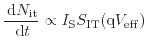
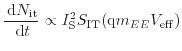
Similar to the approach for the impact-ionization rate in (5.24), Rauch et al. used dominant energies in the model. Here this leads to two discrete maximum energies giving
The emphasis of this modeling approach is again based on the importance of the carrier energy instead of the electric field. To receive an applicable model, the concept of estimating a single peak energy using the effective field instead of calculating the whole distribution function is used to make the calculations more simple.
In the hot-carrier degradation modeling approach by Bravaix et al. [223,244], three different modes depending on the carrier energy can be separated. The first mode is the high carrier energy regime, which usually coincides with lower currents. In this situation the lucky electron model appears valid. This SP degradation is used together with the dominant energy approach at knee points as proposed by Rauch et al. in (6.11). The device life-time in this regime is taken from (6.3) and is estimated with
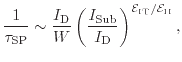 |
(6.13) |
The second mode corresponds to the electron-electron scattering induced degradation, also proposed by Rauch et al. using the formulation shown in (6.12). This leads to the device life-time
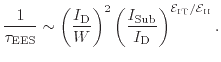 |
(6.14) |
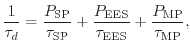
Finally the third mode is relevant at high electron fluxes but with carrier
energies below the threshold energy for the SP process. Similar to the modeling
approach by Hess, the MP mechanism is considered in this model. Furthermore, to
describe the energetics of bond dissociation by this process the concept of the
truncated harmonic oscillator shown in Fig. 6.2 is
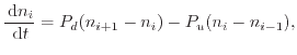
employed. The occupancies ![]() of level
of level ![]() in the oscillator are described
using rate equations. For the first and the following levels the rate equations
are defined as [223]
in the oscillator are described
using rate equations. For the first and the following levels the rate equations
are defined as [223]
 |
(6.15) |
 |
(6.16) |
 |
(6.22) |
![$\displaystyle \frac{1}{\tau_\ensuremath{\mathrm{MP}}} \propto \left[ \ensuremat...
...{W} \right) \right] ^{\ensuremath{\mathcal{E}}_b / \ensuremath{\hbar \omega}} .$](img533.png) |
(6.23) |
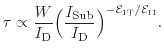
Under real stress/operating conditions all three modes presented contribute to the entire degradation process. Therefore all three regimes are taken into consideration in the Bravaix model. This finally leads to the device life-time
 |
(6.24) |
To summarize, the Bravaix modeling approach combines and enhances the lucky electron model, the electron-electron scattering, and the truncated harmonic oscillator used to model the MP process. This approach has been shown to fit a large range of different devices.
![$\displaystyle \ensuremath{\Delta N_\mathrm{it}}= C_2 \left[ t \frac{\ensuremath...
...suremath{\mathrm{q}}\ensuremath{E_{\mathrm{max}}}\lambda } \Bigr) \right] ^ n .$](img456.png)
![$\displaystyle \ensuremath{\ensuremath{\frac{\ensuremath{ \mathrm{d}}n_N}{\ensuremath{ \mathrm{d}}t}}} = P_u n_{N-1} - P_d \Delta N_\mathrm{it}[H^*] ,$](img518.png)