4.4.3 High-Field Mobility for HD Equations

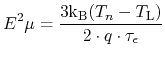
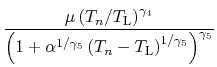
In order to obtain a consistent hydrodynamic mobility expression, the local energy balance equation:

$$E^2\mu=\frac{3 \ensuremath{\mathrm{k}}_\ensuremath{\mathrm{B}}(\ensuremath{T_\ensuremath{n}}-T_\mathrm{L})}{2\cdot q\cdot\tau_\epsilon}$$ (4.72)

is solved for $E(T_\ensuremath{\mathrm{n}})$, which is then inserted into (4.66). This is performed again with $\xi$=1/2 for both models, and with $\beta$=2 for the first model and $\beta$=1 for the second model, respectively. $\tau_\epsilon$ is the energy relaxation time.

Model A:

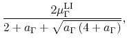
The expression obtained with the chosen values for $\xi$ and $\beta$ is identical with the one proposed by Hänsch et al. [356]. In order to account for NDM effects it is modified by introducing two parameters ($\gamma_4$ and $\gamma_5$) [20]:

$$\ensuremath{\ensuremath{\mu}_{\ensuremath{n}}^{\ensuremath{\mathrm{LIT}}}}(\ensuremath{T_\ensuremath{n}}) = \frac{\mu\left({\ensuremath{T_\ensuremath{n}}}/{T_\mathrm{L}}\rig... ...remath{T_\ensuremath{n}}}-{T_\mathrm{L}}\right)^{1/\gamma_5}\right)^{\gamma_5}}$$ (4.73)

$$\alpha = \frac{3 \ensuremath{\mathrm{k}}_\ensuremath{\mathrm{B}}\ensuremat... ...rm{LI}}}}}{2\mathrm{q}\tau_{\epsilon} \left(v_\ensuremath{\mathrm{f}}\right)^2}$$ (4.74)

In the standard Hänsch model $v_\ensuremath{\mathrm{f}}$ corresponds to the saturation velocity $v_\ensuremath{\mathrm{sat}}$ (as in (4.66)). However, due to the powered temperature term $(\ensuremath{T_\ensuremath{n}}/T_\mathrm{L})^{\gamma_4}$ in the numerator the velocity is steadily decreasing at high-fields. Hence, $v_\ensuremath{\mathrm{f}}$ does not describe the saturation velocity as a physical quantity, although it does affect the high-field transport characteristics. The parameter $\gamma_5$ has a more pronounced effect at low fields, while $\gamma_4$ influences primarily the high-field mobility, though their impact cannot be isolated to a specific field region. The conventional Hänsch model corresponds to the parameter set $\gamma_4=0$, $\gamma_5=1$. However, in order to approximate the simulation and experimental data, a set with $\gamma_4=-0.3$ and $\gamma_5=2.4$ is chosen for GaN (Table 4.10). It delivers good agreement with the velocity-field characteristics obtained using the DD Model B (Fig. 4.16). A similar good match with DD Model A can be achieved for AlN, too (Fig. 4.17). Only for InN it is not possible to model the very strong NDM effect.

Table 4.10: Parameters for HD high-field electron mobility Model A.

	$\gamma_4$	$\gamma_5$
Hänsch	0.0	1.0
GaN	-0.3	2.4
AlN	0.1	3.3

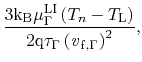
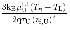
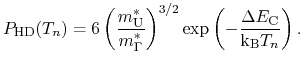
Model B:

Inserting (4.72) into (4.66) with $\xi$=1/2 and $\beta$=2 gives the following expression for the high-field mobility:

$$\mu_\ensuremath{\mathrm{\Gamma}}\left(\ensuremath{T_\ensuremath{n}}\right) = \frac{2 \mu^\ensuremath{\mathrm{LI}}_\ensuremath{\mathrm{\Gamma}}... ...remath{\mathrm{\Gamma}}} \left( 4 + a_{\ensuremath{\mathrm{\Gamma}}} \right)}},$$ (4.75)

$$\mu_\ensuremath{\mathrm{U}}\left(\ensuremath{T_\ensuremath{n}}\right) = \frac{2 \mu^\ensuremath{\mathrm{LI}}_\ensuremath{\mathrm{U}}}{2 +... ...t{a_{\ensuremath{\mathrm{U}}} \left( 4 + a_{\ensuremath{\mathrm{U}}} \right)}},$$ (4.76)

$$a_{\ensuremath{\mathrm{\Gamma}}} = \frac{3 \ensuremath{\mathrm{k}}_\ensuremath{\mathrm{B}}\mu^\ensur... ...remath{\mathrm{\Gamma}} \left({\it v}_\ensuremath{\mathrm{f,\Gamma}}\right)^2},$$ (4.77)

$$a_{\ensuremath{\mathrm{U}}} = \frac{3 \ensuremath{\mathrm{k}}_\ensuremath{\mathrm{B}}\mu^\ensur... ...\tau_\ensuremath{\mathrm{U}} \left({\it v}_\ensuremath{\mathrm{f,U}}\right)^2}.$$ (4.78)

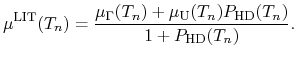
In order to approximate the intervalley transfer at high fields, two sets of $\mu_\ensuremath{\mathrm{v}}$ are used as in DD Model B. In this model too, $v_\ensuremath{\mathrm{f}}$ does not denote the saturation velocity. The weighted mean is built:

$$\mu^\ensuremath{\mathrm{LIT}}(\ensuremath{T_\ensuremath{n}}) = \f... ...suremath{T_\ensuremath{n}})}{1+P_{\mathrm{HD}}(\ensuremath{T_\ensuremath{n}})}.$$ (4.79)

The expression for $P_\ensuremath{\mathrm{HD}}$ is analogous to that for $P_\ensuremath{\mathrm{DD}}$:

$$P_{\mathrm{HD}}(\ensuremath{T_\ensuremath{n}}) = 6\left(\frac{m_{... ...emath{\mathrm{k}}_\ensuremath{\mathrm{B}}\ensuremath{T_\ensuremath{n}}}\right).$$ (4.80)

Fig. 4.19 compares the valley occupancy as a function of the electric field as calculated in this model and MC simulation in GaN. The used parameter setup is the same as for DD Model B (Table 4.9). The only additional values needed, are the scaled energy relaxation times listed in Table 4.11 (the base relaxation times $\tau_{\epsilon, \ensuremath{\mathrm{GaN}}}$, $\tau_{\epsilon, \ensuremath{\mathrm{AlN}}}$, and $\tau_{\epsilon, \ensuremath{\mathrm{InN}}}$ are discussed in Section 4.4.4. An excellent agreement between all models is achieved for GaN (Fig. 4.16). For InN the model can describe the abrupt decay in velocity very well (Fig. 4.18), while the maximum velocity value is slightly higher than the one achieved by the DD model (which is possibly due to the high energy relaxation times used).

Figure 4.19: GaN valley occupancy as a function of the electric field.

While the models deliver consistent results, the two approaches expose some differences. HD Model A is close to already established models and offers a straightforward calibration with only two auxiliary parameters (within a narrow value range). HD Model B is more complex, however, it allows for a more flexible calibration. Its parameters are derived from physical quantities.

Table 4.11: Parameters for the energy relaxation times for HD high-field electron mobility Model B [ps].

	$\tau_\Gamma$	$\tau_\ensuremath{\mathrm{U}}$
GaN	8.0 $\times\tau_{\epsilon,\ensuremath{\mathrm{GaN}}}$	$\tau_{\epsilon, \ensuremath{\mathrm{GaN}}}$
InN	$\tau_{\epsilon, \ensuremath{\mathrm{InN}}}$	0.1 $\times\tau_{\epsilon,\ensuremath{\mathrm{InN}}}$