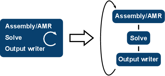
Figure 5.22: The schematic overview of the initial deal.II example (left) and the
proposed decoupling into a loop-based execution graph (right) is shown. For the sake
of simplicity, the sockets are abstracted by single edges.
This section presents application results for each scheduler provided by ViennaX. Due to the nature of ViennaX, the framework can be applied to different fields of CSE. To reflect this fact the discussed examples have been selected accordingly by investigating application scenarios outside of the field of MNDS.
This section discusses adaptive mesh refinement ( AMR), a typical requirement for FE simulations. The general idea is to improve the solution process by locally adapting the mesh during the course of the simulation. Usually, a first solution is computed based on an initial mesh. Based on this solution, the mesh is locally adapted. Typically, a refinement is conducted in regions with large gradients or large curvatures in the solution [162][163]. Increasing the resolution, i.e., adding mesh elements in areas of interest, tends to increase the overall accuracy. The adaptation and solution steps are repeated, until a certain threshold level is reached as indicated by an error estimator [164].
In the following, an example application provided by the deal.II library is investigated [92]. This discussion is followed by depicting a decoupled implementation including simulation results based on ViennaX. Concretely, the step-8 example, dealing with an elasticity problem coupled with an iterative AMR scheme is analyzed and ViennaX’s loop mechanism for modeling the iterative nature of the AMR algorithm is investigated. We analyze the initial implementation, followed by a detailed description of a decoupling scheme.
The initial implementation is based on a single C++ source file, containing a class implementation (ElasticProblem), which provides methods to utilize the deal.II library for solving the elasticity problem.
The subsequent code discussion is based on the class interface instead of the full implementation.
The structure of the class implementation provides an intuitive description of the entire simulation process. The class itself is parameterized via the compile-time template parameter dim (Line 1), indicating the dimensionality of the problem. The run() method (Line 3) drives the overall simulation by performing the iteration process, in turn calling the individual methods required for the computation (Lines 4-8). As the focus of this particular application example is on implementing the AMR algorithm via the ViennaX loop mechanism, the implementation of the run() method deserves closer investigation:
The AMR loop is implemented via the for-loop and the refine_grid method (Lines 3-7). In the first iteration an initial mesh is generated (Lines 4-6). During each loop iteration all steps required for this particular FE simulation are conducted, being the assembly of the linear system of equations and the linear solution process (Lines 8-10).
Concerning the implementation of a decoupled version by using ViennaX, an exemplary decoupling of this particular simulation is schematically depicted in Figure 5.22.
Note that this particular ElasticProblem class implementation had to be slightly altered to allow external access to the data structures and methods. In the following, we focus on the implementation aspects of the Assembly/AMR and Output writer component.
The initialization phase of the Assembly/AMR component is implemented as follows.
We omit the instantiation of the data structures for the mesh, the system matrix, and the load vector. These data structures - kept in the state of the component - are forwarded to the constructor of the sim object. An additional sink socket is used for the loop mechanism (Line 5). A corresponding source socket is used in the last component in the loop sequence, being the Output writer component.
The implementation of the execution part is similar to the original version.
No explicit loop mechanism is required, such as a for-loop, as ViennaX automatically issues a re-execution of the components within the loop. However, to keep track of the loop iteration within the component, the call variable is used (Lines 1,2), replacing the originally utilized cycle loop parameter. The sim object is used to call the respective methods for assembling the linear system of equations (Lines 5-7).
The Output writer component is - additionally to generating the simulation output files - responsible for notifying ViennaX whether to continue the loop. Aside of the obvious sink sockets required to access the result data to be written to a file, this particular component has to provide a complementary source socket to close the loop defined in the initialization phase:
This socket is not required for actual data communication, it is merely required to inform ViennaX that there is a backward-dependence.
The execution phase utilizes the boolean return value to indicate whether the loop has to be continued. In the following example, after six executions, the loop is exited.
In Lines 2,3 ViennaX’s loop break condition is implemented by comparing the call parameter with the intended number of six loop iterations. In this exemplary case, the value is hard coded, however, it can also be implemented in a non-intrusive manner via the data query mechanism provided by ViennaX’s configuration facility (Section 5.3.4). By convention returning true forces ViennaX to exit the loop, whereas returning false triggers a new iteration.
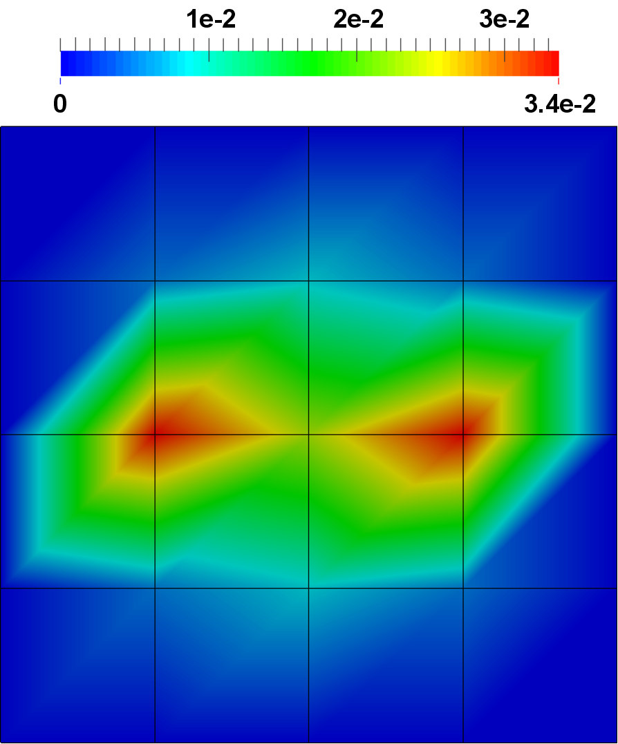
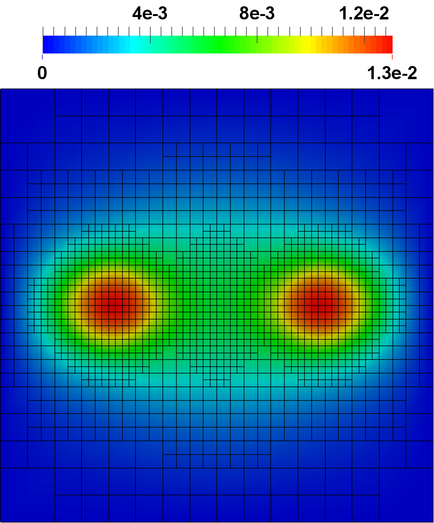
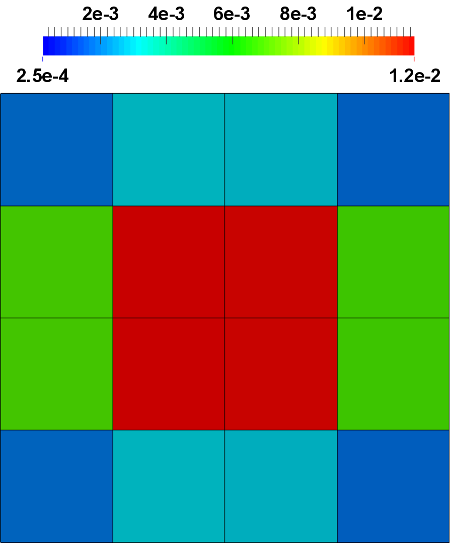
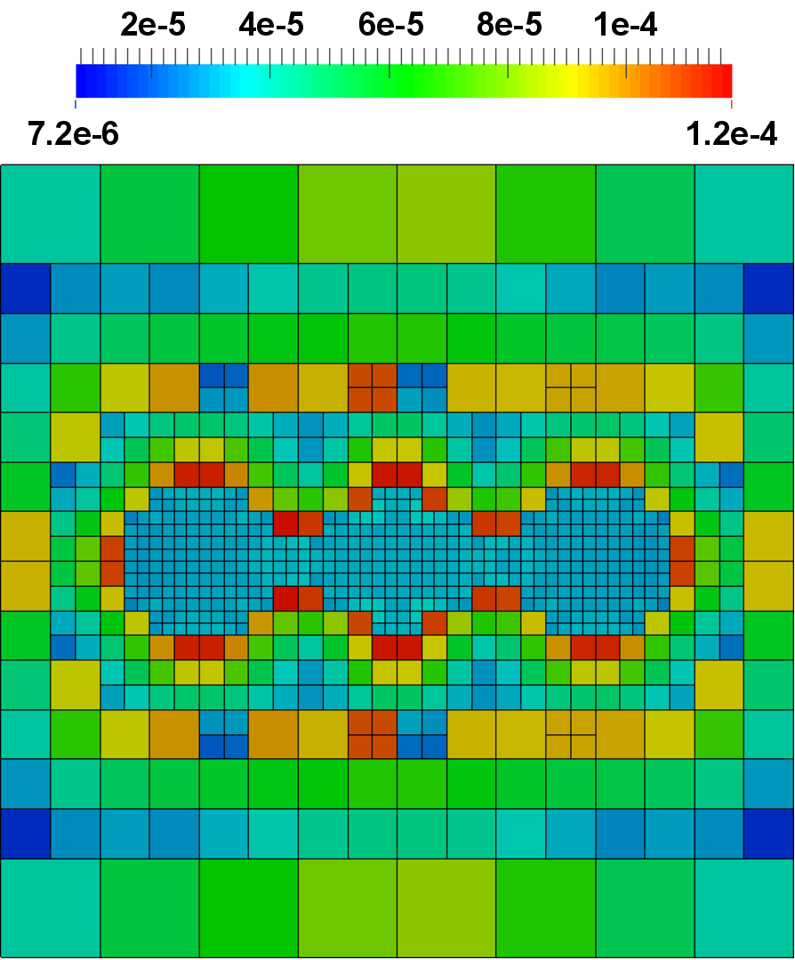
Figure 5.23 depicts exemplary simulation results for a three-dimensional simulation based on the introduced decoupled implementation.
 to
to  . The depicted error estimates
for the sixth iteration would trigger a refinement in the corners in the subsequent
iteration step, as due to the continuing reduction in the error the relative small solution
gradients become relevant.
. The depicted error estimates
for the sixth iteration would trigger a refinement in the corners in the subsequent
iteration step, as due to the continuing reduction in the error the relative small solution
gradients become relevant.
This section investigates the scalability of the DTPM scheduler by a Mandelbrot benchmark as implemented by the FastFlow framework [165][166]. Implementation details of the benchmark are provided as well as performance results. This example has been benchmarked on HECToR [167], a Cray XE6 supercomputer with a Gemini interconnect located at the University of Edinburgh, Scotland, UK.
The DTPM scheduler is used to compute the Mandelbrot set for a partitioned application domain by using different instances of a Mandelbrot plugin responsible for the individual parts. This particular example has been chosen, as the computational effort of computing the Mandelbrot set is inhomogeneously distributed over the application domain. Therefore, the computational load of the individual parts have to be weighted accordingly to improve the scalability.
The partial results are gathered at the end of the simulation, which provides insight into the communication overhead (Figure 5.24). The implementation of the Mandelbrot plugin performs a partitioning of the simulation domain. Thus, each instance is responsible for a subdomain, which is identified by the plugin index. In its essence, this approach follows a data parallel approach, which also shows that the DTPM can be used for such kind of tasks, despite of its inherent focus on task parallelism.
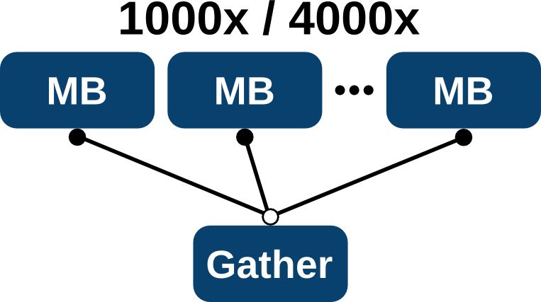
Two different simulation domains have been investigated, being a grid of 1000x1000 and 4000x4000 to demonstrate the influence of varying computational load on the scaling behavior. Each plugin processes one line of the grid, consequently 1000 instances for the smaller and 4000 instances for the larger case have been used.
The following depicts the configuration file for the smaller benchmark.
The clones entry triggers an automatic duplication of the plugin in ViennaX, thus in this
case 1000 instances of the Mandelbrot plugin are generated. The parameters dim and niters
are forwarded to the plugins and relate to the number of grid points in one dimension and the
number of iterations (in this case  iterations are conducted to increase the computational
effort) used in the Mandelbrot algorithm, respectively. The configuration of the larger
benchmark is similar, however, the number of clones and dimensions is increased to 4000,
respectively.
iterations are conducted to increase the computational
effort) used in the Mandelbrot algorithm, respectively. The configuration of the larger
benchmark is similar, however, the number of clones and dimensions is increased to 4000,
respectively.
During the Mandelbrot plugin’s initialization phase, the output socket has to be generated as well as the computational level of the plugin has to be set to balance the computational load over the computational resources. A peculiarity of computing the Mandelbrot set is the fact that the computational load in the center is larger than on the boundary. Therefore, a weighting scheme has been applied to increase the load balancing over the MPI processes. The plugin instances in the center are assigned a higher computational weight (Section 5.3.5) as depicted in the following.
In Line 2 the current plugin ID is extracted, which has been provided by the scheduler
during the preparation phase (Section 5.3.2). As each plugin is responsible for a single line of
the simulation grid, its ID is tested whether it is responsible for the central part. In this case,
the central part is identified by evaluating whether the component is responsible for
the centered  of the grid line, i.e., to be larger equal than
  (
( ) and
smaller equal than
) and
smaller equal than  (
( ) of the grid line dimension. If so, the computational
level is set to a high value, such as
) of the grid line dimension. If so, the computational
level is set to a high value, such as  in this case, to ensure that these center
components are equally spread over the computational resources by the scheduler’s graph
partitioner.
in this case, to ensure that these center
components are equally spread over the computational resources by the scheduler’s graph
partitioner.
As each plugin computes a subset of the simulation result, the output port has to be localized with respect to the plugin instance to generate a unique socket. As already stated, the socket setup has to be placed in the initialization step.
This socket generation method automatically generates sockets of the type Vector and the name vector including an attached string representing the plugin ID, retrieved from the pid method. This approach ensures the generation of a unique source socket for each Mandelbrot plugin instance.
The execution part accesses the data associated with the source socket and uses the data structure to store the computational result. The plugin ID is used as an offset indicating the responsible matrix line which should be processed.
On the receiving side, the Gather plugin’s initialization method generates the required sink sockets using a convenience function.
The above method automatically generates one sink socket for  predecessor
plugins, where
predecessor
plugins, where  represents the current plugin ID. Therefore, all previous output ports
generated by the Mandelbrot plugins can be plugged to the respective sink sockets of the
Gather plugin.
represents the current plugin ID. Therefore, all previous output ports
generated by the Mandelbrot plugins can be plugged to the respective sink sockets of the
Gather plugin.
The execution phase is dominated by a gather method, similar to the MPI counterpart.
The partial results of the  predecessor plugins are stored consecutively in a
vector container, thus forming the result matrix where each entry corresponds to a point on
the two-dimensional simulation grid.
predecessor plugins are stored consecutively in a
vector container, thus forming the result matrix where each entry corresponds to a point on
the two-dimensional simulation grid.
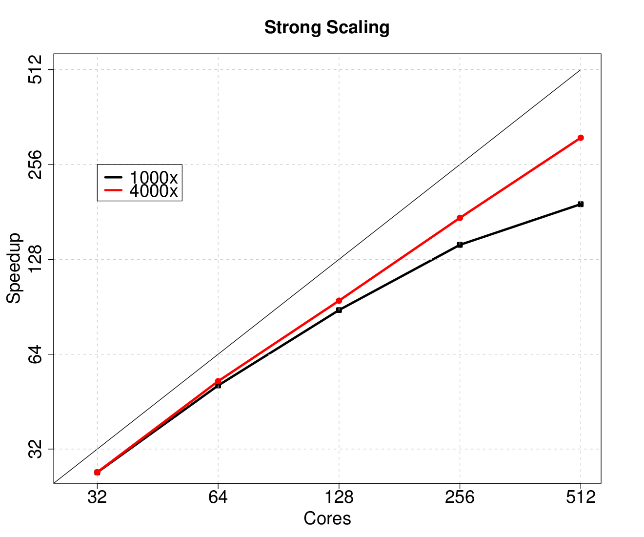
Figure 5.25 depicts the strong scaling results, i.e., a fixed problem size is investigated for
different core numbers. Reasonable scaling is achieved, although communication overhead
and load balancing problems are identifiable already for small core numbers. However,
increasing the computational load on each plugin and the number of plugins to
be processed by the MPI processes further shifts the scaling saturation towards
higher core numbers. For the smaller problem an efficiency of  and for the
larger problem an efficiency of
and for the
larger problem an efficiency of  for 512 cores is achieved. Improving the load
balancing via the plugin weighting approach as well as introducing a hybrid scheduler to
improve communication and computation overhead will further improve the scaling
behavior.
for 512 cores is achieved. Improving the load
balancing via the plugin weighting approach as well as introducing a hybrid scheduler to
improve communication and computation overhead will further improve the scaling
behavior.
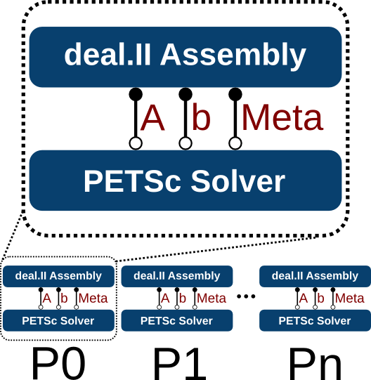
The DDPM scheduler is investigated by comparing the execution performance to a reference implementation provided by the deal.II library [91][92]. This benchmark not only shows that an available implementation using external high-performance libraries can be transferred to the ViennaX framework in a straightforward manner, but also that the execution penalty of using the framework is negligible. Similar to the previous example, HECToR [167] was used as benchmark target.
A large-scale two-dimensional Laplace test case named step-40 of the deal.II library offering 67 million degrees of freedom is considered, which utilizes components representing important aspects of large-scale high performance computing applications [168]. For instance, the data structure holding the mesh and the linear system is fully distributed by using data structures provided by the PETSc library [122] and the p4est library [169][170]. The equations are discretized using biquadratic finite elements and solved using the conjugate gradient method preconditioned by an algebraic multigrid method provided by the Hypre [171] package and accessed via PETSc.
The reference implementation is split into two functional parts, being the assembly by the deal.II library and the solution of the linear system via the PETSc library. Therefore, two plugins have been implemented, which also underlines the reusability feature (Figure 5.26). For instance, the linear solver plugin can be replaced with a different solver without changing the implementations.
The following depicts the configuration file for the benchmark.
The assembly plugin’s initialization phase prepares the distributed data structures as well as provides the source sockets. The data structures required for the computation are generated and kept in the plugin’s state. Therefore, the source sockets are linked to the already available objects, instead of created from scratch during the socket creation. The execute method of the assembler plugin forwards the simulation data structures to the implementation provided by the deal.II example, which performs the actual distributed assembly. This fact underlines the straightforward utilization of already available implementations by ViennaX plugins. The following code snippet gives a basic overview of the assembly plugin’s implementation.
The plugin state holds various data objects (Lines 2-5). The sim objects holds references of the other objects, thus the internals of the simulation class can access the data structures. The source sockets link to already available data objects (Lines 8,9). The simulation grid is generated (Lines 14,15) and the linear system (matrix, rhs) is assembled (Lines 16).
The solver plugin generates the corresponding sink sockets in the initialization part and utilizes the PETSc solver environment in the execution method. As each MPI process holds its own instance of the socket database, the pointers of the distributed data structures are forwarded from the assembler to the solver plugin. The PETSc internals are therefore able to work transparently with the distributed data structures without the need for additional copying operations. The following depicts the crucial parts of the solver plugin’s implementation.
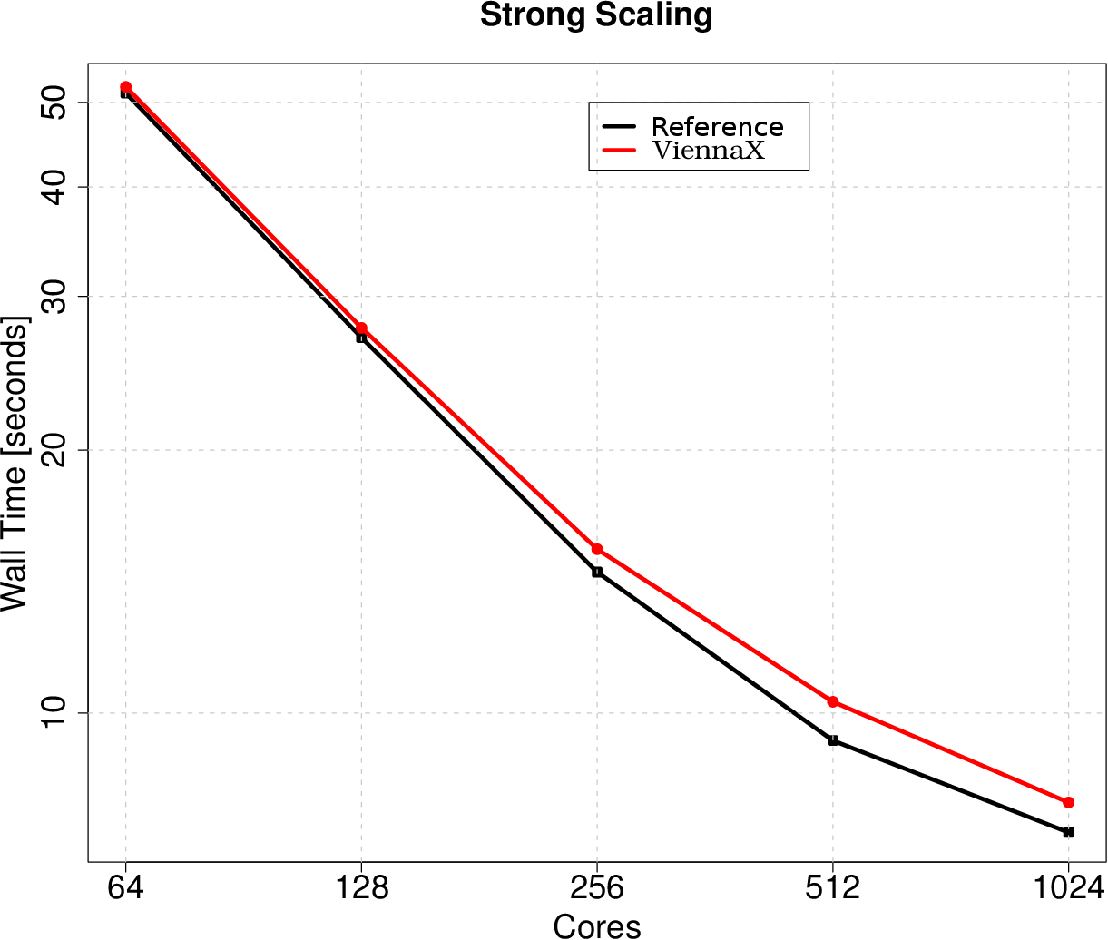
Figure 5.27 compares the execution performance of the ViennaX implementation with the
deal.II reference implementation. A system of 67 million degrees of freedom is investigated,
which due to it’s memory requirements does not fit on one compute node. Generally, excellent
performance is achieved, however, an overall constant performance hit of about
one second for all core numbers is identified. This performance hit is due to the
run-time overhead introduced by the plugin framework, such as the time required to
load the plugins, generate the task graph, and perform virtual function calls. The
relative difference for 1024 cores is around  , however, it is reduced to
  for
64 cores, underlying the fact that the framework’s overhead becomes more and
more negligible for larger run-times. This overhead is acceptable, as the simulations
we are aiming for have run-times way beyond 50 seconds, as is the case for 64
cores.
for
64 cores, underlying the fact that the framework’s overhead becomes more and
more negligible for larger run-times. This overhead is acceptable, as the simulations
we are aiming for have run-times way beyond 50 seconds, as is the case for 64
cores.
Although the relative difference is significant for short run-times, a delay of one second hardly matters in real world, day-to-day applications. On the other hand, accepting this performance hit introduces a significant increase in flexibility to the simulation setup due to the increased reusability of ViennaX’s component approach.