For a problem described by a system of PDEs a local matrix for each element ![]() of the discretization
of the discretization
![]() , nucleus, is constructed.
This nucleus is integrated into the general matrix of the system through a process called assembling.
In this section the assembling algorithm applied in numerical schemes of problems discussed in Chapters 3 and 4 is derived.
, nucleus, is constructed.
This nucleus is integrated into the general matrix of the system through a process called assembling.
In this section the assembling algorithm applied in numerical schemes of problems discussed in Chapters 3 and 4 is derived.
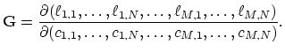
The Jacobi matrix needed for the Newton method in the case of a finite element discretization is,
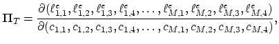 |
(2.42) |
The basic nodal function ![]() , defined at the arbitrary point
, defined at the arbitrary point
![]() is non-zero only on the patch
is non-zero only on the patch ![]() .
Furthermore
.
Furthermore ![]() can be represented as,
can be represented as,
![]() at the point
at the point ![]() and
and
![]() at three other points of the tethraedal element
at three other points of the tethraedal element ![]() .
.
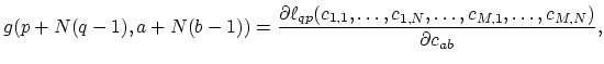
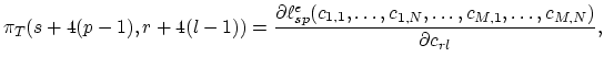
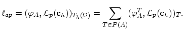
The discrete operators ![]() obtained by testing of
obtained by testing of ![]() -th equation of the system with the basic nodal function
-th equation of the system with the basic nodal function ![]() is,
is,
Obviously in (2.46)
![]() is equal to one of the basic nodal functions
is equal to one of the basic nodal functions
![]() at the element
at the element ![]() .
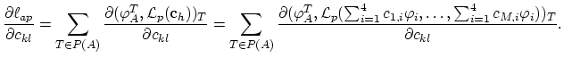
Furthermore, the partial derivative is non-zero only if the
.
Furthermore, the partial derivative is non-zero only if the ![]() stays for one nodal value of
stays for one nodal value of ![]() .
.
We now define the operator ![]() ,
,
![]() ,
, ![]() , which assigns a single global index
, which assigns a single global index ![]() to every local index
to every local index ![]() of vertex belonging to the tethraedal element
of vertex belonging to the tethraedal element ![]() .
The inverse function
.
The inverse function
![]() is also well-defined.
is also well-defined.
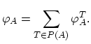
From (2.41), (2.43), and (2.46) we have,
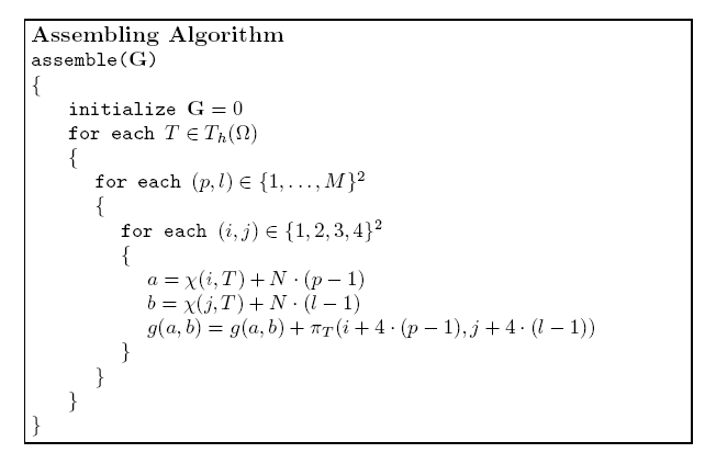
At the end of the assembling process the general matrix
![]() contains the values given by (2.40).
contains the values given by (2.40).