


Next: 2.7 Assembling
Up: 2. Finite Element Method
Previous: 2.5 Finite Element Spaces
Subsections
2.6 Newton Methods
The discretization of the non-linear PDE systems leads to a large system of nonlinear algebraic
equations. There are various methods which solve such systems. Among them the most popular is a Newton method with it's variations.
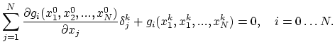
Generally we have a system of N non-linear algebraic equations
 |
(2.32) |
assuming that the functions  have continues first order derivations with respect to
  .
If the values
.
If the values 
 of the
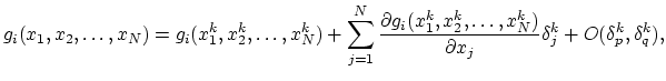
  -th approximate solution are known, we write Taylor series expansion of the functions in the vicinity of
  ,
,
 |
(2.33) |
for
 , where
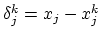 .
By choosing for the exact value
.
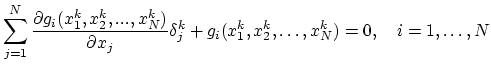
By choosing for the exact value  and neglecting the terms of order
 we have from (2.33)
 |
(2.34) |
The matrix
![$\displaystyle [\mathbf{J}]_{N\times N},\quad J_{ij}=\frac{\partial f_i(x_1^{k}, x_2^{k},\dots,x_{N}^{k})}{\partial x_j},$](img134.png) |
(2.35) |
is called Jacobi matrix. In the case when this matrix is non-singular the linear equation system (2.34) can be solved. Depending on the problem itself different types of linear solvers should be applied [11].
The solutions of the linear system (2.34) are the increments

 and with these increments we can calculate new approximation,
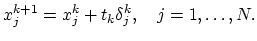 |
(2.36) |
The determination of damping value  is the question of trial and error. The sequences often used for subsequent trials are,
 or or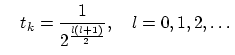 |
(2.37) |
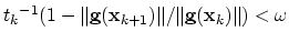
is accepted if the following criterion is fulfilled,
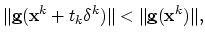 |
(2.38) |
where we use Euclidian norm.
Since the calculation of the Jacobi matrix is a very computer resources-consuming procedure, one can for a number of subsequent Newton iterations also use the same Jacobi matrix (2.35). In that case on obtains,
 |
(2.39) |
The simplified Newton method obviously has a worse convergence behavior.
2.6.4 Damping
In the cases where the convergence of the Newton scheme is attainable only for a very small time steps, methods for the enforcing of the convergence must be applied.
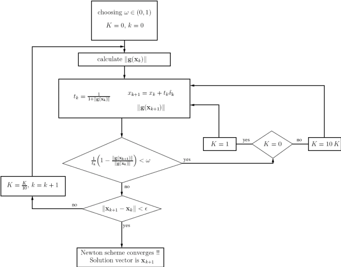
The method which has also successfully been applied in semiconductor device modelling [4], is the so-called Bank-Rose algorithm [12].
Figure 2.3:
Bank-Rose algorithm.
|
The algorithm is represented in Figure 2.3. It controls the behavior of Newton scheme through a damping factor .
The parameter of crucial importance for the algorithm is  . In Figure 2.3 we take
  as initial estimate for
  . Alternatively, we have used
 , where
  is the counter of failed tests
 .
.
The algorithm searchs through the vincinity of the initial solution
 for the shortest path through the attraction region of the Newton scheme to reach the next approximation
 . In the cases when the Bank-Rose algorithm fails the parameter grows infinitely and an improved approximation
is never found.
. In the cases when the Bank-Rose algorithm fails the parameter grows infinitely and an improved approximation
is never found.
Next: 2.7 Assembling
Up: 2. Finite Element Method
Previous: 2.5 Finite Element Spaces
H. Ceric: Numerical Techniques in Modern TCAD