In elasticity theory, an element of volume experiences forces via stresses applied to its surfaces by the surrounding material. Stress is the force per unit area of surface. A complete description of the acting stresses therefore requires not only specification of the magnitude and direction of the force but also of the orientation of the surface, for as the orientation changes so, in general, does the force. Consequently, nine components must be defined to specify the state of stress. They are shown with reference to an elemental cube aligned with the x,y,z axes in Figure 2.2. The component σij, where i and j can be x, y or z, is defined as the force per unit area exerted in the +i direction on a face with outward normal in the +j direction by the material outside upon the material inside. For a face with outward normal in the -j direction, σij is the force per unit area exerted in the -i direction. For example, σyz acts in the positive y direction on the top face and the negative y direction on the bottom face.
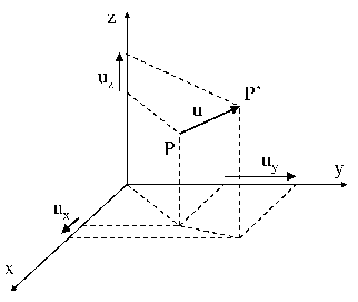
Each point in a strained body is displaced from its original position in the unstrained state. The point displacement is represented by the vector
|
| (2.1) |
Let us consider the body in the condition of mechanical equilibrium. In such situation, no net torques taken about x,y and z axes placed through the center of the cube are present in the element, so that
 | (2.2) |
Thus, the order in which subscripts i and j are written is immaterial. The three components σxx, σyy, σzz are the normal components. From the definition given above, a positive normal stress results in tension and a negative one in compression. The effective pressure acting on a volume element is therefore
p = -  . . | (2.3) |
As a consequence of equilibrium, no net force can act on the element, so that
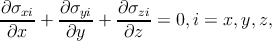 | (2.4) |
equations (2.4) are the so-called equilibrium equations of classic elasticity.
When acted upon by stresses, the body deforms. The displacement u has the components ux, uy, uz representing its projections on the x, y, z axes, as shown in Figure 2.3.
Let us consider now the response to stress. In linear elasticity, the strains are defined in terms of the first derivatives of the displacement components
εij =  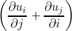 . . | (2.5) |
εxx =  ,εyz = εzy = ,εyz = εzy =  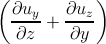 , , | |||
εyy =  ,εzx = εxz = ,εzx = εxz =   , , | |||
εzz =  ,εxy = εyx = ,εxy = εyx =  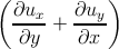 . . | (2.6) |
The strains εxx, εyy, εzz defined in (2.6) are the normal strains. They represent the fractional change in length of elements parallel to the x, y and z axes, respectively, e.g. the length lx of an element in the x direction is changed to lx(1 + εxx).
The volume V of a small volume element is changed by strain to (V + ΔV ) = V (1 + εxx)(1 + εyy)(1 + εzz). In the linear approximation, the fractional change in volume Δ, known as the dilatation, is therefore
 | (2.7) |
Δ is independent of the orientation of the axes x,y,z.
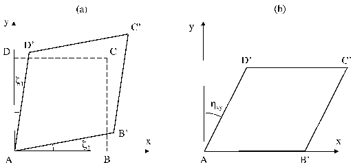
Each component for i≠j is half of the shear strain ηij, which is usually defined in engineering as
| ηij = 2εij,i≠j. | (2.8) |
The shear strain ηxy is related to the angles of shear by the relation
ηxy = ζx + ζy =  + +  . . | (2.9) |
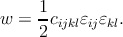
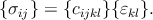
For small distortions (∂ui∕∂xj ≪ 1), each stress component is linearly proportional to each strain. The relationship between stresses and strains in linear approximation is called Hooke’s law. Thus, the stresses depend only on the strains
 | (2.10) |
The coefficients cijkl are the elastic constants, also called stiffness constants. From (2.2) and the relation εkl = εlk, it follows directly that
 | (2.11) |
The combination of the last two relations yields the expression
 | (2.12) |
The further combination of the last equation with (2.4) gives
 | (2.13) |
When a unit volume element deforms reversibly by differential strain increments dεij, the stresses work on the element by an amount
 | (2.14) |
If the deformation is reversible and isothermal, and if the work is restricted to that of elastic deformation, the differential work dw is equal to the differential change in Helmholtz free energy dF of the element
 | (2.15) |
Thus
 | (2.16) |
The free energy is a state function and dF is an exact differential, so that the order of differentiation in the previous equation is immaterial. As a consequence it follows
 | (2.17) |
The strain-energy-density function (the strain energy per unit of volume) is determined by the integration of (2.15)
 | (2.18) |
A typical solution to an elasticity problem involves the determination of the displacements uk from (2.13), given a set of boundary conditions. Stresses and strains then follow from (2.5) and (2.12), and the strain energy follows from (2.18).
Hooke’s law (2.10) written as an equation between matrices becomes
 | (2.19) |
The matrix cijkl is relating the nine elements σij to the nine elements εkl. According to (2.17), the matrix {cijkl} is symmetric. The elastic coefficients are often written in a contracted matrix notation as cmn where m and n are each indices corresponding to a pair of indices ij or kl, according to the following reduction:
| ijorkl112233233112321321, | |||
| morkl123456789. | (2.20) |
| c11 = c1111c12 = c1122 | |||
| c44 = c2323c46 = c2312 | |||
| ...... | (2.21) |
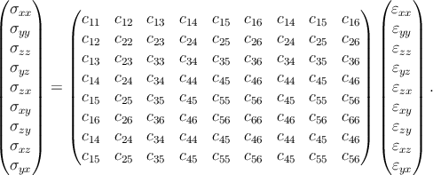 | (2.22) |
Because of the symmetry the previous relation is reduced to the following 6×6 representation
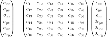 | (2.23) |
The cmn in the 6×6 matrix are the same as the cmn occurring in the 9×9 matrix. The 6×6 matrix is also symmetric. When the axes of reference are rotated, stresses, strains, and elastic constants must be transformed accordingly. Transformations are performed most conveniently in the complete 9×9 scheme. This procedure is described in Section 2.3. For most crystals, the number of independent elastic constants is reduced further from 21 because of crystal symmetry. As an example, only five constants are independent for hexagonal crystals:
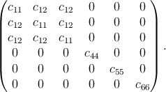 | (2.24) |
For cubic crystals, the independent constants are three:
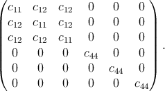 | (2.25) |
For isotropic solids only two material properties – λ and μ, called Lamé constants – are required:
σxx = 2μεxx + λ , , | |||
σyy = 2μεyy + λ , , | |||
σzz = 2μεzz + λ , , | |||
| σxy = 2μεxy,σyz = 2μεyz,σzx = 2μεzx. | (2.26) |
μ =  . . | (2.27) |
| Y | = 1∕s11, | ||
| ν | = -s11∕s12, | ||
| H | = 2p∕Δ. | (2.28) |
Y = 2μ(1 + ν)ν = λ∕2(λ + μ)H =  . . | (2.29) |