4.3.3 The Eigenvalue Solver

For closed boundary conditions (3.103), which represents an eigenvalue equation, must be solved. Such matrix eigenvalue problems arise in many applications of science and engineering. They are given by the matrix equation [177,238]

$$\ensuremath{{\underline{A}}}{\mathbf{x}} = \lambda {\mathbf{x}} \ ,$$ (4.7)

where $\ensuremath{{\underline{A}}}$ is a square $n \times n$ matrix, $\mathbf{x}$ a non-zero $n$ by 1 vector, and $\lambda$ a scalar. The polynomial

$$m(\lambda) = \ensuremath{\mathrm{det}}(\lambda \ensuremath{{\underline{I}}}- \ensuremath{{\underline{A}}}) \ ,$$ (4.8)

where $\ensuremath{{\underline{I}}}$ is the unity matrix, is the characteristical polynomial of $\ensuremath{{\underline{A}}}$. The roots $\lambda_i$ of the equation

$$m(\lambda) = 0$$ (4.9)

are the eigenvalues of $\ensuremath{{\underline{A}}}$. Since the degree of $m(\lambda)$ is $n$, the characteristical polynomial has $n$ roots, and so $\ensuremath{{\underline{A}}}$ has $n$ eigenvalues. A vector $\mathbf{x}_i$ that satisfies

$$\ensuremath{{\underline{A}}}\mathbf{x}_i = \lambda_i \mathbf{x}_i$$ (4.10)

is called an eigenvector of $\ensuremath{{\underline{A}}}$. The matrix $\ensuremath{{\underline{A}}}$ is positive definite, if all eigenvalues are positive, positive semidefinite, if $\lambda_i \ge 0$, negative definite, if all eigenvalues are negative, and negative semidefinite, if $\lambda_i \le 0$. If both positive and negative eigenvalues occur, the matrix is indefinite.

Based on the properties of the matrix $\ensuremath{{\underline{A}}}$, several cases can be distinguished. The matrix $\ensuremath{{\underline{A}}}$ can be HERMITian

$$\begin{array}{ccc} \ensuremath{{\underline{A}}}= \ensuremath{{\underline{A}}}^+&\text{:}&A_{ij} = A_{ji}^\ast \end{array}$$ (4.11)

or non-HERMITian. Furthermore, the matrix elements can be real or complex. A real HERMITian matrix is also denoted a symmetric matrix. A HERMITian matrix has only real eigenvalues, while a non-HERMITian matrix also permits complex eigenvalues. Based on the different cases, different numerical solvers have been used for the solution. Table 4.1 summarizes the different cases.

Table 4.1: Eigenvalues and eigenvectors of matrices with different properties and the numerical solvers used.

Matrix elements	Symmetry	Eigenvalues	Eigenvectors	Solver	Reference
real	HERMITian	real	real	CEPHES	[239]
real	non-HERMITian	complex	complex	EIGCOM	[240]
complex	HERMITian	real	complex	QRIHRM	[240]
complex	non-HERMITian	complex	complex	EIGCOM	[240]

As described in Section 3.6.3.3, calculation of the life times of quasi-bound states requires to find the eigenvalues of the inverse retarded GREEN's function $\ensuremath{{\underline{G}}}^{-1}$ (3.91). Since the coupling entries $\zeta$ and $\xi$ are in general complex, the matrix is complex too. Furthermore, the matrix is not HERMITian. However, it is not possible to straightforwardly calculate the eigenvalues of $\ensuremath{{\underline{G}}}^{-1}$ because the eigenvalue problem is nonlinear [177]: The values of the matrix elements $\zeta$ and $\xi$ depend on the eigenvalue ${\mathcal{E}}$.

Sophisticated methods have been developed to allow an easy solution of this matrix so that the life times can be calculated [241,242,243,244]. First, the closed-boundary HAMILTONian is constructed and the eigenvalues are calculated. In the one-dimensional case the matrix is tridiagonal. It is shown in [245] that in this case, the LU algorithm is advantageous for the calculation of eigenvalues compared to the commonly used QR algorithm which transforms the matrix into an upper HESSENBERG matrix [246]. This is also done by the CEPHES solver. However, since the solver will be used for two- and three-dimensional problems as well, where the LU algorithm shows no advantages, the QR algorithm was applied.

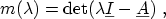
Then, the eigenvalues are filtered so that only the values remain which are located in the considered energy range. These values are then used as initial values for a NEWTON search around the closed-boundary eigenvalue [242,244]. This is motivated by the fact that for ${\mathcal{E}}_i$ being an eigenvalue of $\ensuremath{{\underline{H}}}$ , the determinant

$$m({\mathcal{E}}_i) = \ensuremath{\mathrm{det}}(\ensuremath{{\underline{H}}}-{\mathcal{E}}_i \ensuremath{{\underline{I}}}) = 0$$ (4.12)

must be zero. To find the roots of this equation, a NEWTON search around the closed-boundary eigenvalues ${\mathcal{E}}_i$ is used

$${\mathcal{E}}_{i,j+1} = {\mathcal{E}}_{i, j} - \frac{m({\mathcal{E}}_{i,j})}{m^\prime({\mathcal{E}}_{i,j})} \ ,$$ (4.13)

where $m^\prime({\mathcal{E}})$ denotes the derivative of the determinant

$$m^\prime({\mathcal{E}}) = \frac{\ensuremath {\mathrm{d}}m({\mathcal{E}})}{\ensuremath {\mathrm{d}}{\mathcal{E}}} \ .$$ (4.14)

For a tridiagonal matrix, it is possible to find an analytical expression for $m^\prime({\mathcal{E}})$ [247,248]. For general situations, however, the derivative can only be found numerically by

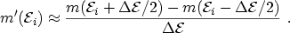$$m^\prime({\mathcal{E}}_i) \approx \frac{m({\mathcal{E}}_i + \Delt... ...}/ 2) - m({\mathcal{E}}_i - \Delta {\mathcal{E}}/ 2)}{\Delta {\mathcal{E}}} \ .$$ (4.15)

This has the advantage that it is not limited to one-dimensional problems but can be applied to any shape of the HAMILTONian.

A. Gehring: Simulation of Tunneling in Semiconductor Devices