) and one parallel (
 ) to a
certain plain is required. The corresponding derivation will be outlined in the
following.
) to a
certain plain is required. The corresponding derivation will be outlined in the
following.
When going from small electron systems, such as atoms and molecules, to large
electron systems, solids for instance, the number of available electron states reaches
high values so that it is best expressed in terms of a density per energy and volume.
In solid state theory the assumption of periodic boundary conditions is frequently
employed and delivers simple first-order approximation of the density of states
(DOS). However, in a few cases, such as tunneling, DOS decomposed in
one energy component perpendicular () and one parallel () to a
certain plain is required. The corresponding derivation will be outlined in the
following.
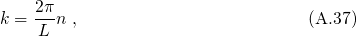
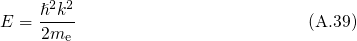
In each direction with periodic boundary conditions, each quantum number  is
directly related to one wavevector
is
directly related to one wavevector  :
:
 is increased, the single quantum states narrows in
the
is increased, the single quantum states narrows in
the  space and
  becomes an continuous quantity. Then the summation over the
single states can be replaced by an integral.
becomes an continuous quantity. Then the summation over the
single states can be replaced by an integral. 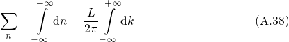
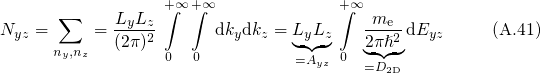
 -direction
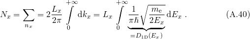
 -plane.
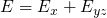
 being the energy in the
  -plane. Combining both solutions yields
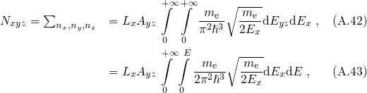
 to
to  with the constraint
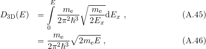
 is performed. The split one/two dimensional DOS is defined as

For the case that the electrons are confined in the  -direction, the number of states
are counted in the following way:
-direction, the number of states
are counted in the following way:
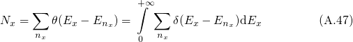
 denotes the quasi-bound states with the quantum number
  . In order
to refer
. In order
to refer  to the unit volume, one must introduce the the square of the
wavefunction.
to the unit volume, one must introduce the the square of the
wavefunction. 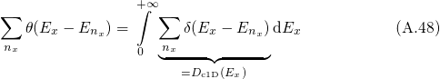
 is multiplied with
  and the same integral transformation as
for the derivation of
and the same integral transformation as
for the derivation of  is performed, one obtains the DOS for an
one-dimensionally confined electronic system:
is performed, one obtains the DOS for an
one-dimensionally confined electronic system: 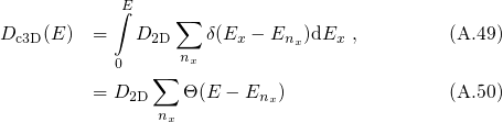
 has been
neglected.
has been
neglected.