 [31, 28, 14, 32, 33, 34, 12, 6]. Therefore, a method has to be found to
convert this measured quantity into a parameter relevant at use-condition, e.g.
[31, 28, 14, 32, 33, 34, 12, 6]. Therefore, a method has to be found to
convert this measured quantity into a parameter relevant at use-condition, e.g.
 .
.
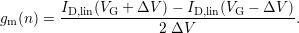
While the MSM-technique was conceived to capture the recovery following
stress as fast as possible, a completely different approach was first
proposed by Denais et al. [28]. In contrast to the discussion of the impact
of fast recovery which cannot be determined prior to the measurement
delay3 ,
the “on-the-fly” method measures the drain current at stress level without ever
interrupting the stress. Due to the experimental setup of never allowing the
device to reach the subthreshold regime during stress, the degradation during
stress can only be monitored via the degradation of the linear drain current
[31, 28, 14, 32, 33, 34, 12, 6]. Therefore, a method has to be found to
convert this measured quantity into a parameter relevant at use-condition, e.g.
.
 -characteristics
is shifted to the right. The change in the subthreshold-slope due to the
increased interface state density affects the physically defined threshold
voltage shift, which depends on the gate voltage, i.e.
-characteristics
is shifted to the right. The change in the subthreshold-slope due to the
increased interface state density affects the physically defined threshold
voltage shift, which depends on the gate voltage, i.e.  . On the
other hand
. On the
other hand  is an empirical quantity, as defined in (2.7). Note that
  is larger than
  in the subthreshold regime.
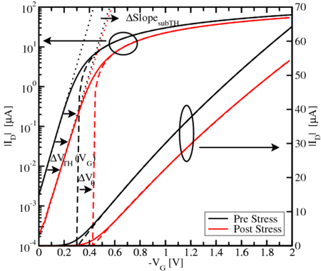
As mentioned in [12], the main problem of the OTF method is that the
 -shift has almost the same effect on the transfer characteristic as the
degradation of the mobility. A shift of
-shift has almost the same effect on the transfer characteristic as the
degradation of the mobility. A shift of  as a consequence of electrically
active defect charges results in a pure vertical shift along the
as a consequence of electrically
active defect charges results in a pure vertical shift along the  -axis. More
precisely this is because defect charges have a direct impact on the surface
potential and hence on the threshold voltage (cf. equation (1.1)). On the other
hand, defects located at the interface cause surface scattering. The thereby
increased channel resistance (lower mobility) yields a lower drain current after
stress and tilts the transfer characteristics. The resulting decrease in
-axis. More
precisely this is because defect charges have a direct impact on the surface
potential and hence on the threshold voltage (cf. equation (1.1)). On the other
hand, defects located at the interface cause surface scattering. The thereby
increased channel resistance (lower mobility) yields a lower drain current after
stress and tilts the transfer characteristics. The resulting decrease in  than
leads to a spurious increase of
than
leads to a spurious increase of  , in addition to the already mentioned
 -shift due to the total defect charge itself. Unfortunately, these two effects
cannot be separated easily in the linear regime, as can be seen in Fig. 2.7.
Due to the saturation of the drain current
-shift due to the total defect charge itself. Unfortunately, these two effects
cannot be separated easily in the linear regime, as can be seen in Fig. 2.7.
Due to the saturation of the drain current  a relative change in
  becomes more and more insensitive to changes in
  with increasing
 .
.
The degradation of  as defined in (1.1) is just attributed to the defect
charges and is independent of the mobility. In contrast to that,
as defined in (1.1) is just attributed to the defect
charges and is independent of the mobility. In contrast to that,  recorded
via the OTF technique does depend on
recorded
via the OTF technique does depend on  [34, 35, 36], just as it reflects the
existence of additional charges (
[34, 35, 36], just as it reflects the
existence of additional charges ( and
and  ). To extract
  the simple
SPICE compact model [37] valid in the linear regime under strong inversion only
is used:
the simple
SPICE compact model [37] valid in the linear regime under strong inversion only
is used:
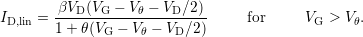 | (2.7) |
While  depends on
  ,
,  models the mobility saturation with
increasing vertical field and
models the mobility saturation with
increasing vertical field and  , the threshold voltage, is obtained by the
intersection of
, the threshold voltage, is obtained by the
intersection of  extrapolated to
  , which is depicted in Fig. 2.7.
Due to the fact that the interface charge depends on the gate voltage
through the occupancy at the interface, as stated in (1.1), the threshold
voltage is not a well defined quantity, i.e.
, which is depicted in Fig. 2.7.
Due to the fact that the interface charge depends on the gate voltage
through the occupancy at the interface, as stated in (1.1), the threshold
voltage is not a well defined quantity, i.e.  [37, 38].
Equation (1.1) uses a physical definition of a threshold voltage, while
[37, 38].
Equation (1.1) uses a physical definition of a threshold voltage, while
 is a purely empirical quantity that yields the best fit to the level 1
model4 .
It can be shown that it is important to provide a large
is a purely empirical quantity that yields the best fit to the level 1
model4 .
It can be shown that it is important to provide a large  -range to get a
reliable extraction of
-range to get a
reliable extraction of  .
.
The main issue with OTF is that as a matter of principle it is not possible to
determine the initial  at
at  , because due to the nonzero
measurement time the device is already stressed, and so the first measurement
yields
, because due to the nonzero
measurement time the device is already stressed, and so the first measurement
yields  . This pre-stressed value is then taken as a reference, which
has a considerable impact on the subsequent extraction of the degradation
[39, 40, 41].
. This pre-stressed value is then taken as a reference, which
has a considerable impact on the subsequent extraction of the degradation
[39, 40, 41].
 -extraction in the
subthreshold-regime,
-extraction in the
subthreshold-regime,  has to be determined under strong inversion.
Lowering the extrapolation range of
has to be determined under strong inversion.
Lowering the extrapolation range of  decreases the possibility of already
pre-stressing the device, but causes an inaccuracy in the thereby determined
decreases the possibility of already
pre-stressing the device, but causes an inaccuracy in the thereby determined
 .
.
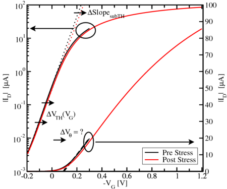
When the  -range is reduced as depicted in Fig. 2.8, at least for the
pre-stressed transfer-characteristic, a value close to the initial value, i.e.
-range is reduced as depicted in Fig. 2.8, at least for the
pre-stressed transfer-characteristic, a value close to the initial value, i.e.
 is obtained. On the other hand this method induces a large error,
which is of the same order of magnitude as
is obtained. On the other hand this method induces a large error,
which is of the same order of magnitude as  itself. Therefore, it
is not feasible to describe the
itself. Therefore, it
is not feasible to describe the  -regime properly by reducing the
 -range.
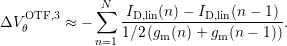
Different OTF models are based on (2.7) and are discussed in Appendix A in
detail. Here the so-called OTF3 after Zhang et al. [34], displayed in Fig. 2.9, will
be described. A change in  can only be converted to
  if the
transconductance
if the
transconductance  , which is defined as the change of the
  over
over  , is
known. To get
, is
known. To get  ,
,  is recorded while slightly varying
  . This
three-point measurement method [28] is indicated in Fig. 2.9 as well and
yields
. This
three-point measurement method [28] is indicated in Fig. 2.9 as well and
yields
 | (2.8) |
By averaging  ,
,  is finally obtained via the sum
 | (2.9) |
In order to prevent a degraded reference of  and
and  , Zhang et al.
suggested to perform the oscillation of
, Zhang et al.
suggested to perform the oscillation of  with a rise and fall time of
  .
Considering such a “degradation-free” reference thus produces a higher amount
of visible
.
Considering such a “degradation-free” reference thus produces a higher amount
of visible  -degradation [42] due to the down-shifted initial value of
 and
and  . Moreover, as
  increases with
  , the OTF-method
measures a higher degradation (
, the OTF-method
measures a higher degradation ( ) compared to the typical
use-condition of a device (
) compared to the typical
use-condition of a device ( ). OTF hence overestimates the
“real” degradation. In contrast the “real” degradation is underestimated, when
the evaluation of
). OTF hence overestimates the
“real” degradation. In contrast the “real” degradation is underestimated, when
the evaluation of  is based on DC transfer characteristics. As a
consequence, the determination of the lifetime is heavily influenced by
either measurement routine. Datasheet conditions on the other hand
should better reflect the real degradation under real use-conditions of
devices.
is based on DC transfer characteristics. As a
consequence, the determination of the lifetime is heavily influenced by
either measurement routine. Datasheet conditions on the other hand
should better reflect the real degradation under real use-conditions of
devices.
Compared to MSM, the biggest advantage of OTF is its recovery-free measurement routine while it is difficult to measure recovery with it, because the OTF technique originally was conceived only to record data in the stress phase of NBTI.
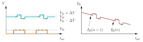
 and their small perturbation
  . The
drain voltage
. The
drain voltage  stays constant during the pulse. Right: The resulting
 whose two points
  and
and  are needed to determine
the degradation of
are needed to determine
the degradation of  . The shift of
  is calculated via (2.8) by using the
modulated
is calculated via (2.8) by using the
modulated  .
.