
Previous: 14.2 Modeling Silicon Self-Interstitial Cluster Formation and Dissolution Up: 14. Inverse Modeling of Silicon Self-Interstitial Cluster Formation Next: 14.4 Summary
Two points from the measurements in [95] were ignored since
they were above the implanted dose. All measurements were viewed as
one vector ![]() . Let
. Let ![]() be the vector of simulation results depending
on the parameters
be the vector of simulation results depending
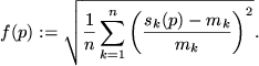
on the parameters ![]() to be identified. The objective function
to be identified. The objective function ![]() to be minimized was the quadratic mean of the element-wise relative
error between a simulated point and a measured point, i.e.,
to be minimized was the quadratic mean of the element-wise relative
error between a simulated point and a measured point, i.e.,
In order to reduce the time needed for the inverse modeling task, the optimization framework SIESTA was used. Its main tasks are optimizing a given objective function and parallelizing the executions of the objective function which usually entails calling simulation tools in a loosely connected cluster of workstations. SIESTA provides several local and global optimizers, the ability to define complicated objective functions, and finally an interface to MATHEMATICA for examining the results. Figure 9.1 shows an overview.
The optimization approach was to first identify reasonable ranges for the variables with great influence, namely energies and exponents. While identifying these ranges suitable starting points for local optimization were found as well. Using these ranges and starting points the optimizations proceeded automatically including all variables.
It was soon found that changing
![]() and
and
![]() did not yield improvements and whenever these variables could be used
by a local optimizer, values very close to
did not yield improvements and whenever these variables could be used
by a local optimizer, values very close to ![]() resulted. The results
described in Table 14.3 and
Figure 14.2 were obtained for the high parameter
set. Similarly we carried out the same computations for the low
parameter set, i.e., TSUPREM-4's default values. These results are
shown in Table 14.3 and
Figure 14.3.
resulted. The results
described in Table 14.3 and
Figure 14.2 were obtained for the high parameter
set. Similarly we carried out the same computations for the low
parameter set, i.e., TSUPREM-4's default values. These results are
shown in Table 14.3 and
Figure 14.3.
Clemens Heitzinger 2003-05-08