13.2 The Basics of the Level Set Method

This section focuses on the basics of the level set method. First the basic ideas of the level set method are outlined. Then the simulation flow, i.e., how the simulation steps are linked in applications, is described. In the following sections the finite difference scheme and advanced concepts like extending the speed function and narrow banding are discussed. The latter two - seemingly unconnected - concepts are combined in the level set algorithm devised in order to arrive at an efficient and precise algorithm.

The idea behind all level set algorithms is to represent the curve or surface in question at a certain time $t$ as the zero level set (with respect to the space variables) of a certain function $u(t,\mathbf{x})$, the so called level set function. Thus the initial surface is the set $\{ \mathbf{x}\mid u(0,\mathbf{x})=0 \}$. Of course the method works for hypersurfaces of arbitrary dimensions, but for applications obviously only curves (two space variables) and surfaces (three space variables) are important.

The evolution of the surface in time is caused by forces or fluxes normal to the surface. The speed of point on the surface normal to the surface will be denoted by $F(t,\mathbf{x})$ and is called the speed function. For points on the zero level set it is usually determined by physical models and in our case by the fluxes of certain gas species and subsequent surface reactions. The speed function $F(t,\mathbf{x})$ generally depends on the time and space variables, and we assume at first that it is defined on the whole simulation domain and for the time interval considered.

The surface at a later time $t_1$ is also the zero level set of the function $u(t,\mathbf{x})$, namely $\{ \mathbf{x}\in\mathbb{R}^n \mid u(t_1,\mathbf{x})=0 \}$. This leads to the level set equation

$$u_{t} + F(t,\mathbf{x}) \Vert \nabla_\mathbf{x}u \Vert = 0,$$

$$u(0,\mathbf{x}) = u_0(\mathbf{x}) ,$$

in the unknown variable $u$, where $u(0,\mathbf{x})$ determines the initial surface. Having solved this equation the zero level set of the solution is the sought curve or surface at all later times. This equation relates the time change to the gradient (with the respect to the spatial variables) via the speed function.

In the numeric application the level set function is represented by values on grid points. During simulations the current surface must be extracted from this grid. This surface extraction step is described in Section 13.4, and appropriate finite difference schemes are given in Section 13.5.

Now in order to apply the level set method a suitable initial function $u(0,\mathbf{x})$ has to be determined first. There are two requirements: first it goes without saying that its zero level set has to be the surface as determined given by the application, and second it should essentially be a linear function at the beginning and throughout the simulation. The second requirement prevents that the absolute value of the gradient of the level set function is too small or too big in the neighborhood of the zero level set. Then high accuracy in the surface extraction steps is ensured and linear interpolation can be used. Of course the second requirement poses demands on the speed function (cf. Section 13.6).

Figure 13.1: This figure shows an example of a signed distance function on the square $[0,1]\times [0,1]$ for a boundary joining the points $(0, \frac 23)$, $(\frac 13, \frac 23)$, $(\frac 13, \frac 13)$, $(\frac 23, \frac 13)$, $(\frac 23, \frac 23)$, and $(1, \frac 23)$. A level set grid with $100\cdot 100$ points was used.

The natural choice for initialization is the signed distance function of a point from the given surface. This function is the common distance function multiplied by $-1$ or $+1$ depending on which side of the surface the point lies in. (In applications the simulation domain is always divided into two areas and the signed distance function is negative for points belonging to the wafer and positive otherwise, or vice versa.) The common distance function of a point $x$ from a set $M$ is then defined by $d(x,M) := \inf_{y\in M} d(x,y)$, where $d$ is usually the Euclidean metric.

The example shown in Figure 13.1 illustrates the initialization of the level set grid using a signed distance function as it is performed by the ELSA simulator (cf. Section 13.8).

The values of the speed function are determined by physical models. The finite difference schemes (cf. Section 13.5) use the values of the speed function at the grid points considered. In topography simulations the physical models determine the speed function only at the zero level set. As outlined earlier they must be extrapolated suitably at grid points not adjacent to the zero level set. How this is done is described in Section 13.3.1 and Section 13.6.

Figure 13.2: Overview of the simulation flow combining transport by physical models and surface evolution using the level set method. The simulation stops when a prescribed time is reached or when a layer of prescribed thickness has been deposited.

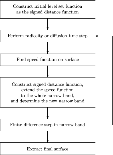Before going into details in the next sections, we close this section by describing the simulation flow of topography simulations as shown in Figure 13.2. First the initial level set grid is calculated as the signed distance function from a given initial surface. In the main loop the surface is extracted and a time step in the physical model is performed. In our applications this means a radiosity of diffusion time step. Thus the speed function at the surface is found. In the next combined step (cf. Section 13.6), a temporary signed distance function is constructed, the speed function is extended, and the new active grid points in a narrow band around the zero level set are determined (cf. Section 13.3). Then the values of the speed function in the active narrow band are used to update the level set grid using a finite difference scheme (cf. Section 13.5).