2.2.1 Heat Flux
It can be observed from various experiments that heat flows from the
hotter to the colder side.
Since the matter that is involved shows a statistical behavior at micro and
nano-scale level in terms of the BROWNian molecular
motion, the previous statement can be formulated as:
The most probable consequence is that heat flows spontaneously from the
hotter to the colder side by diffusion and relaxation mechanisms. This is
exactly the definition of the second law of thermodynamics found
in [73].
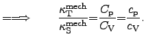
The time derivative of the heat can be expressed by FOURIER's and
LAMBERT's2.12 law, which is equivalent to the
STEFAN2.13-BOLTZMANN law for grey radiators.
These laws consider the spatial temperature gradient
plus the heat flux density due to the surface radiation to the ambient, respectively:
 |
(2.42) |
Here, the first term on the right hand side is determined by FOURIER's law,
where the thermal conductivity tensor is denoted by
 and
and  is
the local temperature in Kelvin. The second term describes LAMBERT's law for
grey radiators, where
is
the local temperature in Kelvin. The second term describes LAMBERT's law for
grey radiators, where
 denotes the STEFAN-BOLTZMANN constant and
 and
and  stand for the ambient and the local surface temperature,
respectively.
The coefficients
stand for the ambient and the local surface temperature,
respectively.
The coefficients
 and
and
 reflect the efficiency of the absorption and the radiation of
the considered surfaces. The ``black body'' has the absorption
and radiation efficiency
reflect the efficiency of the absorption and the radiation of
the considered surfaces. The ``black body'' has the absorption
and radiation efficiency
 .
In most TCAD applications, the radiation can be neglected, except
for areas at the surface of semiconductor devices, for instance, in passivation
layers and heat sinks.
.
In most TCAD applications, the radiation can be neglected, except
for areas at the surface of semiconductor devices, for instance, in passivation
layers and heat sinks.
As the electric and magnetic fields store energy, also the matter
stores heat energy. If heated bodies are put into a colder environment,
they show a certain thermal relaxation behavior.
A possible way to describe this relaxation behavior is to assign a quantity to
each material, where the value of the quantity determines how much energy can be
stored per mass or per mole. This quantity is called specific heat
capacitance2.14.
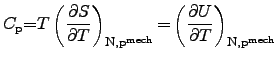
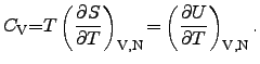
Historically, the heat capacitance is distinguished by two types. The first
one determines the heat capacitance at constant pressure
 and
the second one describes the heat capacitance at constant volume
and
the second one describes the heat capacitance at constant volume
 :
:
 |
|
|
(2.43) |
 |
|
|
(2.44) |
Here, the heat capacitances
and
determine the
change of the internal energy  with regard to the temperature change where
different constraints are applied: constant pressure
and constant volume.
To obtain the specific heat capacitances
with regard to the temperature change where
different constraints are applied: constant pressure
and constant volume.
To obtain the specific heat capacitances
 , the heat capacitances
 are normalized to their involved mass
  :
:
 |
(2.45) |
The unit of the specific heat capacitance is either
 or
or
 according to the type of the mass used
in (2.45) (mass or molar mass).
The different values for the specific heat capacitances of a particular material
can be easily transformed into each other.
according to the type of the mass used
in (2.45) (mass or molar mass).
The different values for the specific heat capacitances of a particular material
can be easily transformed into each other.
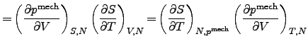
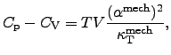
Both heat capacitances of a given material, the one at constant pressure
(cf. (2.43)) and the one at constant volume (cf. (2.44)),
differ from each other by the identity
 |
(2.46) |
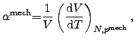
where
 denotes the thermal expansion coefficient at constant pressure, and
 represents the isothermal
compressibility coefficient of the material [76].
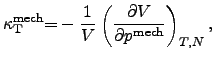
The thermal volume expansion coefficient
and the compressibilities
and
represents the isothermal
compressibility coefficient of the material [76].
The thermal volume expansion coefficient
and the compressibilities
and
 are defined as follows:
Here, the
determines the relative volume change with regard to
temperature changes,
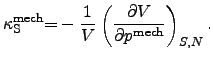
shows the relative isothermal volume change
and
the relative isentropic
volume change with regard to changes of the
local pressure.
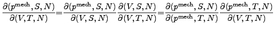
Together with the thermodynamic potentials (2.31) and (2.32) and the
thermodynamic identities (2.36) and (2.37), another correlation between
heat capacitances and compressibilities can be derived by using the chain rule
for differentiation.
The equations (2.50) and (2.51) show the equality of the different
equivalent methods for differentiation according to the chain rules from
LEIBNIZ2.15 and with the previous definitions of the
compressibilities (2.48) and (2.49). Since the isobar
and isochor
heat capacitances describe the same region of matter, their ratio in (2.51)
is the same as for the corresponding specific heat capacitances.
For
isotropic and temperature-independent materials, the left hand side
of (2.9) becomes  times the LAPLACEian2.16operator and (2.9) can be written as
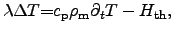 |
(2.53) |
where the maximum of the thermal conductivity has been published for
carbo-nano-tubes (CNTs) and nano wires as
 in [77,78]. In comparison to
that, the thermal conductivity of diamond is typically in the range of
in [77,78]. In comparison to
that, the thermal conductivity of diamond is typically in the range of
 [79,80].
To determine the proper heat generation term
 for a particular problem,
several proposals have been made for semiconductor and interconnect models. The
simplest model is to calculate the power loss with the local electrical field
for a particular problem,
several proposals have been made for semiconductor and interconnect models. The
simplest model is to calculate the power loss with the local electrical field
 and the resulting local current density
 [81,82] by
 |
(2.54) |
where
and
can be calculated using the appropriate models to
describe the observed behavior of the electrical field and the electrical
current density.
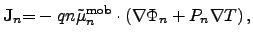
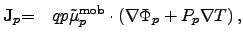
In order to account for the current densities
 and
and
 appropriately, the SEEBECK2.17 effect
has to be considered as well, where the phenomenological
semiconductor current equations [62,66] can be enhanced by
appropriately, the SEEBECK2.17 effect
has to be considered as well, where the phenomenological
semiconductor current equations [62,66] can be enhanced by
 |
|
|
(2.55) |
 |
|
|
(2.56) |
where  and
and  represent the carrier concentrations for electrons and holes,
 and
and
 denote the mobility tensors for
electrons and holes, and
denote the mobility tensors for
electrons and holes, and  and
and  are the SEEBECK
coefficients for electrons and holes.
The quantities
are the SEEBECK
coefficients for electrons and holes.
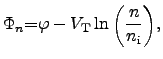
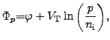
The quantities  and
and  represent the
quasi-FERMI2.18 potentials for electrons and holes in
semiconductor materials:
represent the
quasi-FERMI2.18 potentials for electrons and holes in
semiconductor materials:
 |
|
|
(2.57) |
 |
|
|
(2.58) |
where  denotes the local potential,
 is the thermal voltage according to
 , and
, and
 denotes the intrinsic carrier concentration of the semiconductor
material.
denotes the intrinsic carrier concentration of the semiconductor
material.
For semiconductor devices, the
temperature
is often assumed to be the lattice temperature of the semiconductor crystal
since the carriers and the lattice can be considered as two systems in thermal
quasi equilibrium [66].
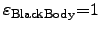
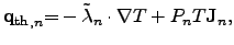
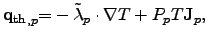
For a rigorous treatment of
the SEEBECK effect, also the FOURIER law for the heat conduction
equation (2.8) has to be adapted to
 |
|
|
(2.59) |
 |
|
|
(2.60) |
where the first part is due to FOURIER's law and the second part due to
SEEBECK's effect.
Stefan Holzer
2007-11-19