2.2.2 ONSAGER's Theorem
A rigorous description of thermal influences on the
electrical current and vice versa has been presented by
ONSAGER2.19 in 1931 [83,84].
His theory discusses the relations of reciprocity of reversible and irreversible processes,
where the coupling of the electrical and the thermal subsystems are investigated.
For instance, if the electrical driving force is denoted as
 and the
thermodynamic driving force
and the
thermodynamic driving force
 is expressed as,
 |
(2.61) |
where  has been identified as the absolute temperature by CARNOT2.20 [61,85],
the corresponding equation system can be formulated with independent equations as
has been identified as the absolute temperature by CARNOT2.20 [61,85],
the corresponding equation system can be formulated with independent equations as
 |
|
|
(2.62) |
 |
|
|
(2.63) |
where  and
and  are the electrical resistivity and the thermal ``heat
resistance'', respectively. The heat resistance is also called thermal resistance
are the electrical resistivity and the thermal ``heat
resistance'', respectively. The heat resistance is also called thermal resistance
 in this thesis. The quantities
 and
and
 are the
electrical and the thermal current, respectively. The thermal current density
is
also called heat flow density
are the
electrical and the thermal current, respectively. The thermal current density
is
also called heat flow density
 .
Several thermodynamic experiments over the last 150 years have shown that the
electrical current is not independent of the temperature. Therefore, equations
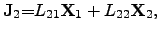
(2.62) and (2.63) are coupled. Introducing the
standard notation, these equations can be adapted by cross coefficients
.
Several thermodynamic experiments over the last 150 years have shown that the
electrical current is not independent of the temperature. Therefore, equations
(2.62) and (2.63) are coupled. Introducing the
standard notation, these equations can be adapted by cross coefficients  and
and  and represent the ONSAGER relations
 |
|
|
(2.64) |
 |
|
|
(2.65) |
For this equation system, THOMSON proposed the relation
 |
(2.66) |
which is also called ``reciprocity theorem'' of the ONSAGER relations.
However, (2.66) implies that this relation follows from
symmetric principles of thermodynamic theory. Hence, the reciprocity theorem
neglects the loss during heat conduction and energy conversion
and relation (2.66) assumes a balanced energy flow between the
two subsystems. Thus, a steady stage is assumed with the request
of (2.66) [61], where equilibrium conditions are
applicable only within short range.
The principle of microscopic reversibility in (2.66) is less
general than the second fundamental law of thermodynamics [83].
For further investigated coupled systems, the currents  may have
different signs due to the different directions of the energy flows. Therefore,
(2.66) is not sufficient enough to fulfill the second law of
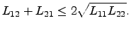
thermodynamics. Hence,
the necessary condition for the equation system consisting of
(2.64) and (2.65) to guarantee the second law with
may have
different signs due to the different directions of the energy flows. Therefore,
(2.66) is not sufficient enough to fulfill the second law of
thermodynamics. Hence,
the necessary condition for the equation system consisting of
(2.64) and (2.65) to guarantee the second law with
 yields
 |
(2.67) |
This necessary condition has been originally proposed by BOLTZMANN
in 1887 [86].
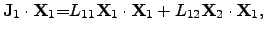
Writing the ONSAGER relations (2.64) and (2.65) as functions of
driving forces

 |
|
|
(2.68) |
 |
|
|
(2.69) |
where the necessary condition of type (2.67) remains valid accordingly for
 as
as
 |
(2.70) |
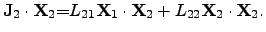
To consider the ONSAGER relations in terms of energy, (2.68)
and (2.69) can be multiplied by
 and
,
respectively, leading to
and
,
respectively, leading to
 |
|
|
(2.71) |
 |
|
|
(2.72) |
These equations represent the products of the driving forces
and
displacements of types of flow
 .
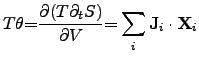
The result of (2.71) and (2.72) can be described as the
dissipated energy per volume and per time and reads
.
The result of (2.71) and (2.72) can be described as the
dissipated energy per volume and per time and reads
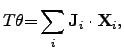 |
(2.73) |
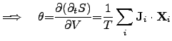
where  is the entropy generation rate per unit volume and follows from the second
law of thermodynamics (2.35)
is the entropy generation rate per unit volume and follows from the second
law of thermodynamics (2.35)
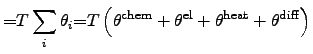
where the entropy generation rate
 can be determined by the sum of
the power densities of all contributing subsystems.
Hereby, the parts of the sums can be identified as the power densities of the
participating systems which are determined by chemical reactions, the power loss
due to heat transfer and JOULE's self-heating, and the power loss due to
diffusion processes.
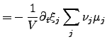
The power density of chemical reactions can be expressed by scalar-valued
quantities as
can be determined by the sum of
the power densities of all contributing subsystems.
Hereby, the parts of the sums can be identified as the power densities of the
participating systems which are determined by chemical reactions, the power loss
due to heat transfer and JOULE's self-heating, and the power loss due to
diffusion processes.
The power density of chemical reactions can be expressed by scalar-valued
quantities as
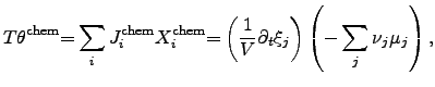 |
(2.77) |
where
 is determined by the chemical reaction rate
 per
unit volume
per
unit volume  . The chemical driving force is represented by
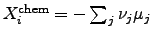 , where
  denotes the
chemical potential and
denotes the
chemical potential and  the stoichiometric coefficient of the
participating atom.
The electrical power density can be identified by
the stoichiometric coefficient of the
participating atom.
The electrical power density can be identified by
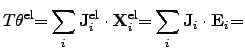 |
|
|
|
 |
|
|
(2.78) |
where
 and
and
 are the electrical current density and the
electrical field, respectively. The electric field can be expressed by the spatial
gradient of an electrical potential
are the electrical current density and the
electrical field, respectively. The electric field can be expressed by the spatial
gradient of an electrical potential  .
For electro-magnetical subsystems, the power density has to be appropriately
adapted as discussed in Section 2.2.3.
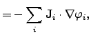
Another important contribution to the global entropy increase is the power loss
due to thermal heat flow, which can be expressed in terms of (2.73)
by
.
For electro-magnetical subsystems, the power density has to be appropriately
adapted as discussed in Section 2.2.3.
Another important contribution to the global entropy increase is the power loss
due to thermal heat flow, which can be expressed in terms of (2.73)
by
 |
|
|
|
 |
|
|
(2.79) |
where
represents the local heat flux density.
The second term in (2.79) depicts the thermal driving force
according to FOURIER's empirical law.
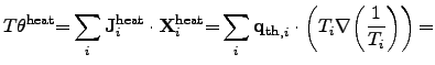
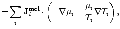
For diffusion processes, the power density can be identified as
 |
|
|
|
 |
|
|
(2.80) |
where
 is the mole number per unit area and time of the
contributing species
is the mole number per unit area and time of the
contributing species  .
The driving force of diffusion processes is determined by the gradient of the
chemical potential and by the gradient of the temperature.
.
The driving force of diffusion processes is determined by the gradient of the
chemical potential and by the gradient of the temperature.
Since the power density of diffusion processes has been determined for no
external forces, an extension for the applied electrical field has to be made by
introducing an additional term that depicts the force acting on charged
particles inside the simulation domain. Hence, equation (2.80)
has to be modified as
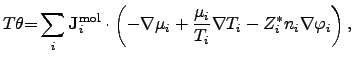 |
(2.81) |
where  is the effective valence charge of the species
,
is the effective valence charge of the species
,  is the
species concentration per mole, and
is the
species concentration per mole, and  is the corresponding electrical
potential.
is the corresponding electrical
potential.
To conclude ONSAGER's thermodynamical treatment, the overall power density is
thus given by the sum of the power densities of all contributing subsystems as
where the thermodynamic power density  is determined by the
contributing chemical reactions, the electrical burden, heat flows, and molar
diffusion processes.
is determined by the
contributing chemical reactions, the electrical burden, heat flows, and molar
diffusion processes.
Stefan Holzer
2007-11-19