This thesis deals with mechanical phenomena mainly caused by electro-thermal
stress conditions. Since the electrical burden produces heat and the heat
non-negligible volume expansion, the mechanical part has to be considered as
well.
The basic equation used for TCAD purposes is HOOKE's2.27 law
which has been originally introduced by the words ``Ut tensio sic
vis''2.28. The corresponding
formula reads
 |
(2.107) |
where the absolute value of the applied force  to a body is proportional to
its elongation
to a body is proportional to
its elongation  . Here the constant
  determines the stiffness
of the body.
More generally, HOOKE's law can be formulated for local quantities in a body
where the local stress tensor
determines the stiffness
of the body.
More generally, HOOKE's law can be formulated for local quantities in a body
where the local stress tensor
 is associated to the
GREEN2.29 tensor (local strain tensor)
is associated to the
GREEN2.29 tensor (local strain tensor)
 for a given
body by
for a given
body by
 |
|
|
(2.108) |
 |
|
|
(2.109) |
where the proportionality factor is determined by the
 -rank
stiffness tensor
-rank
stiffness tensor  and the strain is defined according to CAUCHY2.30via local displacements
 |
(2.110) |
where
 is the displacement or deformation vector and
 the local position.
Using the VOIGT2.31 notation [96,97,98],
the ranks of the tensors involved in (2.108) can be reduced due to
the symmetry of the material and due to the symmetry according to energy conservation
laws [59]. Thus, the number of independent tensor entities
reduces from  to
to  by material symmetry and further reduces to
  mutual
independent tensor entities due to energy
conservation [96,59].
Therefore, equation (2.108) can be expressed
as
mutual
independent tensor entities due to energy
conservation [96,59].
Therefore, equation (2.108) can be expressed
as
 |
(2.111) |
where
 and
and
 are the vector-valued quantities for the
mechanical stress and strain in the VOIGT notation, respectively.
Furthermore,
are the vector-valued quantities for the
mechanical stress and strain in the VOIGT notation, respectively.
Furthermore,  represents the stiffness matrix of
 rank also in the VOIGT notation.
In TCAD applications of modern devices it is often sufficient to deal with
static stresses, only. In that cases, the speed of involved particles can be
neglected [99].
The mechanical equations
have to fulfill general conservations laws [96,97] for energy,
momentum, angular momentum, and mass.
Thus, the mechanical subsystem can be described by the
local conservation laws of energy, momentum, and mass
In (2.112)
the local energy density is denoted by  , the energy flux density by
 , and
, and
 represents the mechanical power
density. The latter equation represents the mechanical analogon of the POYNTING
vector.
Equation (2.113) is the momentum conservation equation, where
represents the mechanical power
density. The latter equation represents the mechanical analogon of the POYNTING
vector.
Equation (2.113) is the momentum conservation equation, where
 is the momentum density,
 is the local force density,
 the velocity of the moving particles, and
 is the momentum flux density which is often called pressure tensor.
Equation (2.114) presents the local mass continuity equation, where the
specific mass density is denoted as
is the momentum flux density which is often called pressure tensor.
Equation (2.114) presents the local mass continuity equation, where the
specific mass density is denoted as
 .
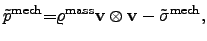
If mass fluxes have to be considered, for instance in electro-migration
analysis, the kinetic pressure tensor
becomes
.
If mass fluxes have to be considered, for instance in electro-migration
analysis, the kinetic pressure tensor
becomes
 |
(2.115) |
where the specific mass density is denoted by
,
is the stress
tensor, and
is the speed of the moving particles.
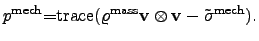
Later on,
can be also used as a scalar-valued quantity
 when the simplified VOIGT notation is used:
 |
(2.116) |
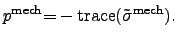
If the flux of mass has not to be considered, the associated velocity of the
particles becomes
 and the hydrostatic pressure can be determined
by
and the hydrostatic pressure can be determined
by
 |
(2.117) |
The definitions of hydrostatic pressure
in (2.116)
and (2.117) can be used as a metric which provides a possibility to
visualize, to compare within measurements, or to define a figure of merit in an
optimization loop [100].
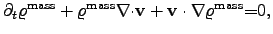
If moving particles are considered, the mechanical analogon to the electrical
continuity equation is the mass continuity equation (2.114) and can be
treated with the EULERian2.32 continuity
equation [96]
 |
(2.118) |
which is the mass conservation equation (2.114).
A mathematical coupling between the mass flux and the mechanical stress can be
obtain by using the first law for continuity mechanics from
CAUCHY
 |
(2.119) |
where the
represents the externally applied force density.
Stefan Holzer
2007-11-19