2.3.2 Transmission Function

An important material property of a semiconductor is the density of states (DOS). The DOS of a system indicates the number of states per energy interval and per volume. The analytical descriptions for the DOS of an isotropic material can be easily calculated [53,32]. However, the bandstructure of materials is not always isotropic. Especially in low dimensional materials, the electronic structure is affected by confinement and several complex features appear. Numerical approaches in the calculation of the DOS are necessary, and depending on the sophistication of the numerical model employed, most of the electronic structure properties are usually captured accurately [32].

If $\varepsilon_{\alpha}(\vec{k})$ denotes the bandstructure, where $\alpha$ indicates the band number and $\vec{k}$ is the wave vector, then the number of states with energy smaller than $E$ is [32]:

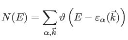$$N(E)=\sum_{\alpha,\vec{k}} \vartheta \left( E-\varepsilon_{\alpha}(\vec{k})\right)$$ (2.38)

where $\vartheta$ is the unit step function. Therefore, the DOS is calculated by:

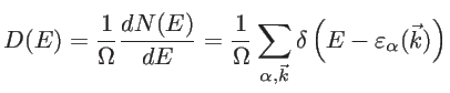$$D(E)=\frac{1}{\Omega}\frac{dN(E)}{dE}=\frac{1}{\Omega}\sum_{\alpha,\vec{k}} \delta \left( E-\varepsilon_{\alpha}(\vec{k})\right)$$ (2.39)

where $\delta$ is the Dirac-delta function and $\Omega$ the volume. In the case of two- and one-dimensional systems, the volume is replaced by the area $A$ and the length $L$ , respectively. For numerical stability, in order to obtain a continuous DOS, a broadening through a Lorentzian function is employed, instead of the sharp delta function [32]:

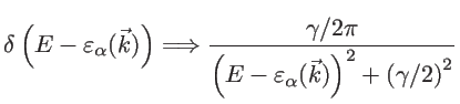$$\delta \left( E-\varepsilon_{\alpha}(\vec{k})\right)\Longrightarr... ...2\pi}{\left( E-\varepsilon_{\alpha}(\vec{k})\right)^2+\left( \gamma/2\right)^2}$$ (2.40)

where the broadening parameter to be used $\gamma=0.3~\mathrm{meV}$ is similar to the energy spacing between the various states.

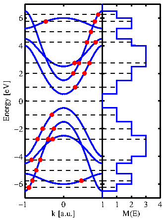
Figure 2.7: A typical bandstructue and its corresponding number of modes at some energies.

Another important ballistic quantity is the number of subbands or modes. The transmission function $\overline{T}_{\mathrm{el}}(E)$ is, indeed, the multiplication of the number of modes $M(E)$ and transmission probability $T_{\mathrm{el}}(E)$ :

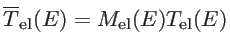$$\overline{T}_{\mathrm{el}}(E)=M_{\mathrm{el}}(E) T_{\mathrm{el}}(E)$$ (2.41)

In the ballistic regime, the transmission of each subband is one and, therefore, the number of modes represents the ballistic transmission function. To calculate $M_{\mathrm{el}}(E)$ , it is enough to count the number of modes at a given energy:

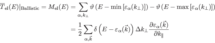$$\begin{split}\overline{T}_{\mathrm{el}}(E)\vert _{\mathrm{Bal... ...repsilon_{\alpha}(\vec{k})}{\partial k_{\parallel}} \end{split}$$ (2.42)

where $k_{\perp}$ refers to the wave vector component perpendicular to the transport direction and $k_{\parallel}$ to the wave vector component parallel to the transport direction [52,32,30]. Finally, we mention that the group velocity of an electron in a Bloch state is defined as:

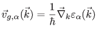$$\vec{v}_{g,\alpha}(\vec{k})=\frac{1}{\hbar} \vec{\nabla}_{k} \varepsilon_{\alpha} ( \vec{k} )$$ (2.43)

The prefactor $1/2$ in Eq. 2.42 is used since only states with positive group velocities along the transport direction contribute to the conductance:

$$v_{g,\parallel}=\frac{1}{\hbar} \frac{\partial \varepsilon_{\alpha}(\vec{k})}{\partial k_{\parallel}}>0$$ (2.44)

A typical test-case bandstructure and the way of counting the modes is shown in Fig. 2.7.

In the presence of scattering processes, the transmission probability $T_{\mathrm{el}}$ is less than one. To include scattering effects, several transport approaches are commonly used, such as the linearized Boltzmann transport equation, Monte Carlo simulations for solutions of the Boltzmann equation beyond the linear regime, the scattering-matrix method, and the non-equilibrium Green's function (NEGF) method. From all these methods, only the quantum mechanical NEGF method is able to capture the wave nature of electrons. It is also able to take into account the atomistic details of actual boundaries and surfaces and capture boundary scattering in nanostructures [32,54].

We use the NEGF method to study the effect of boundary scattering on the electronic transmission of one-dimensional graphene-based structures. For these simulations, the system is assumed to consist of three sections: the channel, the source contact, and the drain contact. The boundary scattering mechanism is introduced in the channel by physically distorting the boundaries. The contacts are assumed to be pristine and always at equilibrium. To describe the electronic structure of this system, the Hamiltonian matrix is set up using the third nearest neighbor tight-binding method as described in Sec. 2.1.1. The system can be described using the following matrices [32]: i) $[H_{ch}]_{n_{ch}\times n_d}$ is the Hamiltonian matrix of the channel (device Hamiltonian), ii) $[H_{s/d}]_{n_R\times n_R}$ is the Hamiltonian of the source and drain contacts (reservoirs), and iii) the couplings between the unit cells of the device $[\tau_{s/d}]_{n_d\times n_R}$ . Here, $n_{ch}$ and $n_R$ indicate the number of basis orbitals in the channel and contacts, respectively. In the NEFG method, the contacts are described through the self-energy matrices:

$$\Sigma_{s/d}=\tau_{s/d} G_{s/d} \tau_{s/d}^{\dagger}$$ (2.45)

where

$$G_{s/d}=\left[ EI_{n_R\times n_R} -H_{s/d} +i0^{+}I_{n_R\times n_R}\right]^{-1}$$ (2.46)

is the Green's function for the isolated contacts. $I_{n_R\times n_R}$ is an identity matrix of the size of the contacts. The device (channel) Green's function can then be calculated as [32]:

$$G_{ch}(E)=\left[ EI_{n_d\times n_d} -H_{ch} -\Sigma_s -\Sigma_d \right]^{-1}$$ (2.47)

The transmission function can be calculated as:

$$\overline{T}_{\mathrm{el}}(E)=\mathrm{Trace}[\Gamma_s G_{ch} \Gamma_d G_{ch}]$$ (2.48)

where the broadening matrices are defined as:

$$\Gamma_{s/d}=i\left[ \Sigma_{s/d}-\Sigma_{s/d}^{\dagger} \right]$$ (2.49)

Finally, it is worth mentioning that in NEGF formalism scattering processes are included using some additional self-energy functions [32]. However, in this thesis, we only investigate the effect of roughness scattering (as the dominant scattering event in nanostructures), which can directly be included in $H_{ch}$ through missing atoms at the edges.