


 Previous: 2.1 The Boltzmann Poisson
Up: 2.1 The Boltzmann Poisson
Next: 2.1.2 Poisson Equation
Previous: 2.1 The Boltzmann Poisson
Up: 2.1 The Boltzmann Poisson
Next: 2.1.2 Poisson Equation
For a distribution function
 where
where
 is the position,
 is the wave vector and
  is the time
the Boltzmann equation for parabolic energy bands reads
is the time
the Boltzmann equation for parabolic energy bands reads
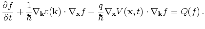 |
(2.1) |
Here
 is the given energy band diagram,
  is the
electrostatic potential and
is the
electrostatic potential and  is the carrier charge (negative
for electrons). The independent variables
are
is the carrier charge (negative
for electrons). The independent variables
are
 ,
,
,
,
 .
.
We define the group velocity

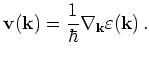 |
(2.2) |
For now we restrict ourselves to parabolic bands. Then
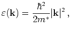 |
(2.3) |
with effective mass  and
and
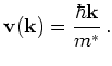 |
(2.4) |
The momentum
 is defined as
 |
(2.5) |
Using the group velocity
the Boltzmann equation becomes
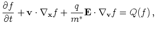 |
(2.6) |
where we introduced the electrical field
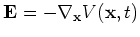 .
.
Previous: 2.1 The Boltzmann Poisson
Up: 2.1 The Boltzmann Poisson
Next: 2.1.2 Poisson Equation
R. Kosik: Numerical Challenges on the Road to NanoTCAD