So far we have assumed parabolicity in our derivations. The non-parabolic case is discussed in broad detail in [GJK+04]. Here we restrict ourselves to a short summary.
First we have to decide on a set of solution variables and express the remaining moments via closure relations. A second issue is the choice of weight functions and indeed different sets of weight functions have been frequently used.
As solution variables we choose the unknowns
![]() and
and
![]() , that is the moments
, that is the moments ![]() .
In the non-parabolic case we use the following set
of weight functions:
.
In the non-parabolic case we use the following set
of weight functions:
| (2.43) |
| (2.44) |
The product ![]() ,
which appears in the calculation, has units of energy.
In the derivation above, valid for the parabolic case,
we used the fact that (under the isotropy condition) moments of
the form
,
which appears in the calculation, has units of energy.
In the derivation above, valid for the parabolic case,
we used the fact that (under the isotropy condition) moments of
the form
![]() can be reduced to
can be reduced to
![]() . For non-parabolic bands this is no longer the
case.
. For non-parabolic bands this is no longer the
case.
Due to the choice of solution variables the balance
equations are independent of the band structure
model and the same as in the parabolic case.
For the flux equations a simple method to close the
equations in the solution variables is to introduce
correction factors ![]() , see [GJK+04].
This gives the
following modified equations:
, see [GJK+04].
This gives the
following modified equations:
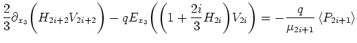 |
(2.45) |
The correction factors ![]() can be tabulated as a function
of temperature and doping extracted from bulk Monte Carlo
simulations.
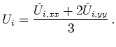
We define
can be tabulated as a function
of temperature and doping extracted from bulk Monte Carlo
simulations.
We define ![]() by
by
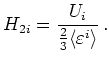 |
(2.46) |
| (2.47) |
 |
(2.48) |
![]()
![]()
![]()
![]() Previous: 2.2.2.2 Odd Moments
Up: 2.2.2 Hierarchy of Moment
Next: 2.2.3 Closure Problem
Previous: 2.2.2.2 Odd Moments
Up: 2.2.2 Hierarchy of Moment
Next: 2.2.3 Closure Problem