Depending on the set of constraints different classes of distribution functions are obtained. For our applications the constraints can be divided in two classes: the first consists of a set of determined moments, the second consists of additional constraints (related to the isotropicity condition) on the distribution functions.
Here we will only study the closure from the reduction conditions 2.40. It is also possibly to study the closures from other constraints, e.g., isotropic symmetric part or the shifting (linear-isotropic) assumption, but the corresponding families cannot be described using elementary functions.
The maximum entropy closure from the reduction conditions is easily achieved, by noting that they determine additional moments, which have to be included in the ansatz.
Hence we get the following family of distributions
| (3.8) |
Then the 7 free parameters have to be determined from the 5 known moments plus the two moments which are additionally known from the reduction conditions.
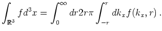
If a function ![]() is written as
is written as
| (3.9) |
 |
(3.10) |
![]()
![]()
![]()
![]() Previous: 3.2 Maximum Entropy Closure
Up: 3.2 Maximum Entropy Closure
Next: 3.2.2 Critique and Modifications
Previous: 3.2 Maximum Entropy Closure
Up: 3.2 Maximum Entropy Closure
Next: 3.2.2 Critique and Modifications