3.4 Gaussian Invariant Closure

If the first three moments of a one-dimensional distribution function are known, a unique normal distribution with parameters $\mu$ and $\sigma$ is defined. Similarly, by assuming that the diffusion approximation holds (that is, the odd moments are assumed to be small) $M_0$ and $M_2$ fix a distribution function in three dimensions, which gives the relation

$$\frac{M_0 M_4}{M_2^2} = \frac{5}{3} .$$ (3.18)

Hence, naturally, the assumption of gaussianity gives a closure for the hierarchy of moment equations at order 4.

For probability distributions ($M_0 = 1$) the kurtosis $\kappa$ is defined as

$$\kappa = \frac{\tilde{M}_4}{\tilde{M}_2^2} .$$ (3.19)

Note that here $\tilde{M}_2,\tilde{M}_4$ denote the central moments of a one-dimensional probability distribution. The kurtosis is one invariant of the class of Maxwellian distributions. Deviations from this constant value are measures of nongaussianity.

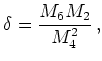
Other invariants exist and can be used to define closure relations. One such family of invariants was used in [GKGS01] to express the sixth moment as a function of the lower moments.

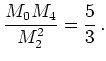
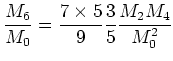
Similar to the kurtosis is the dimensionless quantity $\beta$

$$\beta = \frac{\langle \varepsilon^2 \rangle}{\langle \varepsilon^2 \rangle_M}$$ (3.20)

Here the subscript $M$ denotes the Maxwellian distribution with local temperature $T_n$. In terms of moments $\beta$ is given by Equation 3.14.

Then we approximate $M_6$ by ([Gri02], p.24)

$$<tex2html_comment_mark>601 M_6 = \frac{7 \times 5}{9} M_0 \bigg(\frac{M_2}{M_0}\bigg)^3 \beta^c \, .$$ (3.21)

In terms of moments this closure is written as

$$M_6 = \frac{7 \times 5}{9} M_0^{c-2} M_2^{3-2c} M_4^c \bigg(\frac{3}{5}\bigg)^c .$$ (3.22)

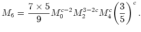
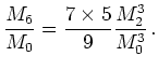
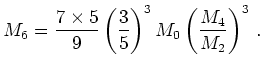
For this type of closure the sixth moment is a rational function in the even moments. When this is combined with the use of mobilities to describe the scattering integral this method can be easily implemented by extending an existing drift-diffusion code.

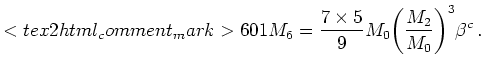
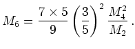
A suitable value of $c$ is found by comparison with Monte Carlo data. This approach was developed in [GKGS01], [Gri02], where $c$ was assumed integer.

For $c=0$ we get $M_6$ from a Maxwellian with temperature $T_n$ by the relation:

$$\frac{M_6}{M_0} = \frac{7 \times 5}{9} \frac{M_2^3}{M_0^3} .$$ (3.23)

For $c=1$ a dimensionless parameter

$$\gamma = \frac{M_0 M_6}{M_2 M_4}$$ (3.24)

can be introduced. The closure becomes

$$\frac{M_6}{M_0} = \frac{7 \times 5}{9} \frac{3}{5} \frac{M_2 M_4}{M_0^2}$$ (3.25)

This closure was studied in [SYT⁺96].

For $c=2$ we get another Gaussian invariant and introduce a parameter $\delta$ as

$$\delta = \frac{M_6 M_2}{M_4^2} ,$$ (3.26)

which is (up to a constant factor) the quotient between $\gamma$ and $\beta$. The definition of $\delta$ is a generalization of the kurtosis. This gives the closure

$$M_6 = \frac{7 \times 5}{9} \left(\frac{3}{5}\right)^2 \frac{M_4^2}{M_2} .$$ (3.27)

Note that only for this value of $c$ the closure does not depend on $M_0$.

Finally, for $c=3$ we get

$$M_6 = \frac{7 \times 5}{9} \left(\frac{3}{5}\right)^3 M_0 \left(\frac{M_4}{M_2}\right)^3 .$$ (3.28)

It is only for the value of $c=3$ that the sixth moment goes with the first power of $M_0$.

In general the given moments $M_0, M_2$, and $M_4$ cannot be represented as moments of a Gaussian distribution. Yet all closures of the family impose some type of gaussianity condition on the moments of the distribution function.

As the generalized invariant approach does not make an ansatz for the distribution function $f$ it has the advantage that the domain of skewness and kurtosis which can be represented is in principle not restricted, which improves the fourth order closure 3.18.