6.1.2 Hydrodynamical Formulation

The hydrodynamic model, originally proposed by Madelung [Mad27], provides a classical picture for quantum dynamics, namely, that of the flow of an indestructible probability fluid.

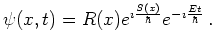
Mathematically it consists in representing $\psi$ using polar coordinates as

$$\psi(x,t) = R(x,t) e^{\imath S(x,t)/\hbar} .$$ (6.17)

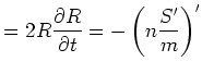
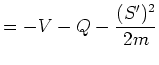
Substituting this ansatz into the time-dependent Schrödinger equation with constant mass and separating into real and imaginary parts, gives two equations:

$$\frac{\partial n}{\partial t} = 2 R \frac{\partial R}{\partial t} = -\left(n \frac{S'}{m}\right)'$$ (6.18)

$$\frac{\partial S}{\partial t} = -V -Q - \frac{(S')^2}{2m}$$ (6.19)

where we introduced the quantum density $n(x) = R(x)^2$ and the so-called quantum potential $Q$:

$$Q = -\frac{\hbar^2}{2} \frac{(\frac{R'}{m})'}{R} .$$ (6.20)

In these formulas the prime $'$ denotes the one-dimensional space derivative.

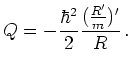
The quantum potential arises from the kinetic energy of the Schrödinger equation and creates the ``self-field''. Alternatively $n Q$ can be seen as pressure in a hydrodynamical Navier-Stokes interpretation [Har66], which is related to Nelson's stochastic interpretation of quantum mechanics.

In the classical limit (e.g., WKB approximation [Kol00], [Sch69]) Equation 6.19 becomes the Hamilton-Jacobi equation with principal function $S$.

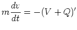
With the identification of the velocity

$$v = \frac{S'}{m}$$ (6.21)

and the flux

$$j = n v$$ (6.22)

the Equation 6.18 becomes the continuity equation

$$\frac{\partial n}{\partial t} = - j'$$ (6.23)

and the second equation can be rewritten as an equation of motion (assuming constant mass $m$)

$$m \frac{dv}{dt} = -(V + Q)'$$ (6.24)

where in the last equation $\frac{d}{dt}$ denotes the Lagrangian (also called ``convective'') derivative [Bit00], [SRV89].

In the deBroglie-Bohm interpretation of quantum mechanics a particle has a sharp position $x(t)$ at each time moving along a fluid trajectory determined by Equation 6.25 (with $v = \frac{dx(t)}{dt}$). Evolution in the Bohm picture is ``sharp'', but the initial condition given by the initial location of the particle is a distribution. Tunneling is explained by lowering the barrier through the additional Bohm potential $Q$. This is a hidden variables theory which singles out position as a preferred variable. The same can be done for other observables, see [Vin00].

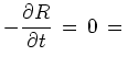
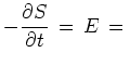
In the stationary case we have

$$\psi(x, t) = R(x) e^{\imath \frac{S(x)}{\hbar}} e^{-\imath \frac{E t}{\hbar}} .$$ (6.25)

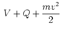
This gives $S(x,t) = S(x) - Et$ and

$$- \frac{\partial R}{\partial t} = 0 = j' \quad$$ (6.26)

$$- \frac{\partial S}{\partial t} = E = V + Q + \frac{mv^2}{2}$$ (6.27)

which expresses conservation of particle number and of energy.

The hydrodynamical formulation can be extended to the mixed state case and was used for quantum mechanical simulation in [BM02], [LW99], [Dal03], [Bit00].

It is pointed out in [Wal94], that the hydrodynamical formulation needs an additional quantization constraint for equivalence with the ``standard'' Schrödinger equation.