6.1.3 The Riccati and Prüfer Equation

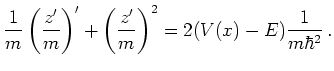
The Riccati equation was used in [Bit00] as a numerically more suitable variant of the hydrodynamical formulation.

Set

$$z = \ln \psi .$$ (6.28)

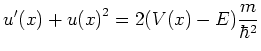
With this the stationary Schrödinger equation

$$- \frac{\hbar^2}{2} \Bigl(\frac{\psi'}{m}\Bigr)' + V(x) \psi = E \psi,\quad 0 < x < L$$

becomes

$$\frac{1}{m} \left( \frac{z'}{m} \right)' + \left( \frac{z'}{m} \right)^2 = 2 (V(x) - E) \frac{1}{m \hbar^2} .$$ (6.29)

By the substitution

$$\frac{z'}{m} = y$$ (6.30)

it reduces to a nonlinear first order equation. For constant mass $m$ and $z' = u$ we get

$$u'(x) + {u(x)}^2 = 2 (V(x) - E) \frac{m}{\hbar^2}$$ (6.31)

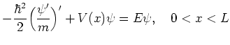This type of equation is known as Riccati equation [MR96]. The Riccati equation plays an important role in control theory and has a rich theory of its own. Separation of Equation 6.30 into real and imaginary part recovers the hydrodynamical equation for the phase $S$ as equation for the imaginary part of $z$.

Another alternative formulation of the Schrödinger equation, which is closely related to the Riccati equation, is the Prüfer equation. The Prüfer transformation is a useful tool in the qualitative theory of second order Sturm-Liouville differential equations [BD01]. In the case of the Schrödinger equation with constant mass $m$ it is introduced in the following way: Define complex quantities $q,p$

$$q = \psi$$ (6.32)

$$p = \frac{1}{m} \frac{d \psi}{dx} .$$ (6.33)

Introducing the transformation

$$q = r \cos(\alpha) ,$$ (6.34)

$$p = r \sin (\alpha) ,$$ (6.35)

with complex $r$, and $\alpha$ we get from the Schrödinger equation and from the defining equation for $p$ (6.34)

$$\frac{\hbar^2}{2} (r' \sin(\alpha) + \alpha' r \cos(\alpha)) = (E - V(x))r \cos(\alpha)$$ (6.36)

$$\frac{1}{m} (r' \cos(\alpha) - \alpha' r \sin(\alpha)) = r \sin (\alpha) .$$ (6.37)

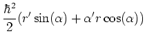
Respective multiplication of these equations with $-\sin(\alpha)$ and $\cos(\alpha)$ and adding the resulting equations yields (after elimination of $r$):

$$\alpha' = \frac{2 m}{\hbar^2}(V(x) - E) \cos^2(\alpha) - \sin^2(\alpha) .$$ (6.38)

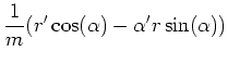
So the equation for the angular variable separates. For $r$ we get:

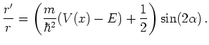$$\frac{r'}{r} = \bigg( \frac{m}{\hbar^2}(V(x) - E) + \frac{1}{2}\bigg) \sin(2\alpha) .$$ (6.39)

The link to the original Riccati idea is immediate. If $\alpha$ is a solution to the Prüfer equation, then $u = \tan(\alpha)$ is a solution to the Riccati Equation 6.32. The advantage of the Prüfer equation (6.39) over the traditional Riccati equation is that it can be solved for arbitrary $\alpha$ without leading to singularities, as is the case with nodes ( $\psi(x) = 0$) in the Riccati equation. The Schrödinger, Riccati and Prüfer equation will be investigated numerically in Section 7.1.3.