There are numerical issues with the
Wigner transform
so that we would like to avoid this task. Instead we will now
define a distribution which in one dimension classically
approximates the phase space distribution.
We want our distribution to reproduce exactly the marginal
expectation values for ![]() ,
, ![]() and
and ![]() . Other local
expectation values are not necessarily reproduced correctly.
. Other local
expectation values are not necessarily reproduced correctly.
Carrier, current, and energy marginal densities
can be directly calculated from the Schrödinger function
![]() respectively the hydrodynamical
quantities
respectively the hydrodynamical
quantities
![]() with
with
![]() .
Instead of the densities
.
Instead of the densities
![]() we
prefer to work with the marginal
we
prefer to work with the marginal ![]() -distributions for
the in the case of constant mass
equivalent set of ``local'' observables
-distributions for
the in the case of constant mass
equivalent set of ``local'' observables
![]() , where
, where
![]() denotes the identity operator.
denotes the identity operator.
Introducing the variable
| (6.65) |
we get the marginal expectation values
(using the split of the energy operator as in Equation 6.63)
for a pure state
![]() :
:
| (6.66) | ||
 |
(6.67) | |
| (6.68) |
To define a corresponding classical phase
space distribution function
![]() we assume that for a wave function
we assume that for a wave function ![]() the corresponding
distribution w(x,p) for each
the corresponding
distribution w(x,p) for each ![]() consists of left (up)
and right (down) going modes, i.e.:
consists of left (up)
and right (down) going modes, i.e.:
This assumption makes sense in cases,
in which the classical problem has a similar
property. Such is the case for the scattering problems
and the open Schrödinger equation which we consider
in Section 7.1.
In this case particles are injected with a fixed
momentum ![]() from one electrode and condition 6.70
is fulfilled exactly. In the electrodes we have
a superposition of transmitted and reflected modes.
from one electrode and condition 6.70
is fulfilled exactly. In the electrodes we have
a superposition of transmitted and reflected modes.
From the ansatz 6.70 we can calculate the classical quantities:
| (6.70) | ||
| (6.71) | ||
| (6.72) |
Classically ![]() and
and ![]() are always positive quantities.
Equating the marginal expectation values from
the wave function and from the
``classical'' distribution function
are always positive quantities.
Equating the marginal expectation values from
the wave function and from the
``classical'' distribution function ![]() we get the system of equations:
we get the system of equations:
| (6.73) |
 |
(6.74) |
| (6.75) |
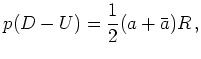
From the last equation we get
 |
(6.76) |
which reduces the system of equations to
 |
(6.77) | |
| (6.78) |
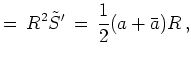
with the solution
 |
(6.79) |
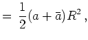
 |
(6.80) |
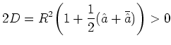
with
 |
(6.81) |
The coefficients ![]() and
and ![]() are positive values between
0 and
are positive values between
0 and ![]() as has to be the case for proper probabilities.
To sum up: Our (1+1)-dimensional
distribution function has the property that it
is positive and reproduces the moments up to an order
as has to be the case for proper probabilities.
To sum up: Our (1+1)-dimensional
distribution function has the property that it
is positive and reproduces the moments up to an order ![]() correctly.
correctly.
![]()
![]()
![]()
![]() Previous: 6.2.5 A Caveat on
Up: 6.2 Quantum Mechanics in
Next: 6.2.7 Quantum Propagators and
Previous: 6.2.5 A Caveat on
Up: 6.2 Quantum Mechanics in
Next: 6.2.7 Quantum Propagators and