7.1.2.1 Schrödinger: Transparent BCs

The idea of transparent boundary conditions is to model the problem in the unbounded domain. Then one imposes boundary conditions such that the solution from the finite problem is exactly the same as the solution from the unbounded problem restricted to the simulation domain.

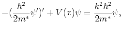
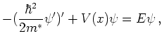
We now apply this procedure to the stationary Schrödinger equation

$$- (\frac{\hbar^2}{2 m^{*}} \psi')' + V(x) \psi = E \psi ,$$

where we have an incoming right-traveling stationary wave $\psi^{\mathrm{in}}(x) = e^{\imath kx}$ coming from $- \infty$ entering the device region via the left lead. We assume $k > 0$ and $E = \frac{k^2 \hbar^2}{2m^{*}}$.

The device region is represented by the spatial interval $(0,L)$. We assume that $V$ is constant in the leads:

$$V(x) = 0, \mbox{$x < 0$} ,$$

$$V(x) = V_L, \mbox{$x > L$} .$$

In general we have $V_L \neq 0$. In approaches which use the Fourier transform of $V$ this creates numerical problems as the Fourier transform of $V$ behaves essentially like the Fourier transform of a Heaviside step function and exists only in the sense of distributions.

Part of the incoming plane wave is reflected by the potential and goes back to $- \infty$:

$$\psi^r(x) = R_k e^{-\imath kx}, \qquad x \le 0 .$$ (7.2)

Note that $\psi^r = \psi - \psi^{in}$ (and not $\psi$) has to fulfill the absorbing boundary conditions, i.e., we really have inhomogeneous transparent boundary conditions on the left boundary.

The other part of the wave is transmitted and travels to $+\infty$. With $V = 0$ in the left lead the energy of the incoming particle is $E = \frac{k^2 \hbar^2}{2m^{*}}$. Using the fact that energy is conserved we get

$$\psi^t(x) = T_k e^{\imath \sqrt{k^2 - 2 m^{*} V_L / \hbar^2} x}, \mbox{$x > L$.}$$ (7.3)

for the transmitted wave.

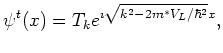
In the left lead the steady state solution hence takes the form

$$\psi(x) = \psi^{\mathrm{in}}(x) + \psi^r(x), \mbox{$x > L$} .$$ (7.4)

The three subproblems (one for each domain) are coupled by the assumption that $\psi$, $\hbar \psi'/m^*(x)$ are continuous across the artificial boundaries at $x = 0$ and $x = L$. This allows us to eliminate the a-priorily unknown coefficients $R_k$ and $T_k$. For a fixed wave vector $k$ of the incoming wave this yields the boundary value problem (BVP):

$$- (\frac{\hbar^2}{2 m^{*}} \psi')' + V(x) \psi = \frac{k^2 \hbar^2}{2 m^{*}} \psi, \quad 0 < x < L,$$

$$\psi'(0) + \imath k \psi(0) = 2 \imath k, \quad x = 0,$$ (7.5)

$$\psi'(L) = \imath \sqrt{k^2 - 2 m^{*} V_L / \hbar^2} \psi(L), \quad x = L .$$

We note that the boundary conditions contain the spectral parameter $k$ and are non-homogenous as the amplitude of the incoming wave packet is normalized to unity. The Fourier transform of the wave $\psi$ exists only in the sense of distributions.

It is important to find a good numerical discretization of the transparent BCs. This is done in [Arn01] where the discretization is determined in such a way that there are no reflections in the case of a flat potential and a homogenous incoming wave.

We have only derived transparent boundary conditions for the stationary case. The same can also be done for the transient Schrödinger equation. However in this case the boundary conditions become non-local in time $t$ and the equation ``has a memory''. Recently Ehrhardt and Arnold [AES03] derived a discretization which they claim to be feasible for numerical simulation.