The boundary conditions given by 7.5 translate to
 |
(7.6) | ||
| (7.7) |
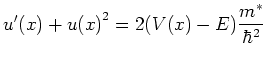
If we set ![]() we get (with constant mass in the electrodes)
we get (with constant mass in the electrodes)
| (7.9) |
Solving Equation 7.8 fixes ![]() . The
value of
. The
value of ![]() is fixed up to
an additive constant
is fixed up to
an additive constant ![]() , which is then determined
by the second boundary condition. For the Prüfer
Equation 6.39 we get the Dirichlet boundary condition
, which is then determined
by the second boundary condition. For the Prüfer
Equation 6.39 we get the Dirichlet boundary condition
| (7.10) |
We stress that with inflow boundary conditions the wave
function ![]() cannot have nodes, hence in
this case the Riccati equation has an everywhere defined solution.
The main advantage
with respect to the Schrödinger equation is that it
is a (nonlinear) first order equation with a Dirichlet
boundary condition.
cannot have nodes, hence in
this case the Riccati equation has an everywhere defined solution.
The main advantage
with respect to the Schrödinger equation is that it
is a (nonlinear) first order equation with a Dirichlet
boundary condition.
We have implemented both the Prüfer and the Riccati equation as an alternative to the Schrödinger equation. The results are reviewed in the next section.
![]()
![]()
![]()
![]() Previous: 7.1.2.1 Schrödinger: Transparent BCs
Up: 7.1.2 Absorbing Boundary Conditions
Next: 7.1.3 Comparison: Schrödinger, Riccati
Previous: 7.1.2.1 Schrödinger: Transparent BCs
Up: 7.1.2 Absorbing Boundary Conditions
Next: 7.1.3 Comparison: Schrödinger, Riccati