The following is based on Apsley's work [19]. We will derive a formula for both the conductivity's temperature as well as its field dependence in the case of a Gaussian density of states mirroring the molecular disorder. We assume that (i) the localized states are distributed randomly in both space and energy, (ii) the states are occupied according to the Fermi-Dirac statistics, (iii) both hops upwards and hops downwards are regarded, (iv) the state energies are uncorrelated, and (v) the electric field may assume any value. Finally, the mobility's concentration dependence is discussed.
| (2.20) |
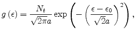
In various disordered systems, a Gaussian density of states has been used to describe the hopping transport in band tails.
 |
(2.22) |
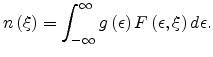
Let
![]() be the normalized Fermi-Dirac distribution
function. Then the carrier concentration can be written as
be the normalized Fermi-Dirac distribution
function. Then the carrier concentration can be written as
 |
(2.23) |
![$\displaystyle N\left(T,\beta,R,\epsilon_i\right)=\int_0^{\pi}\int_0^{R}\int_{-\...
...ight)\right]\frac{1}{8\alpha^3} 2\pi R^{ '2}\sin\theta d\epsilon_jdR 'd\theta$](img271.png) |
According to Mott, ![]() will be the value of the radius in the hopping
space for which only one available vacant site is enclosed [72]. In
other words,
will be the value of the radius in the hopping
space for which only one available vacant site is enclosed [72]. In
other words, ![]() can be obtained by solving the equation
can be obtained by solving the equation
 |
(2.26) |
![$\displaystyle I_1=\int_0^{\pi}\sin\theta\cos\theta d\theta\int_{\epsilon_j-R_{n...
...\frac{R_{nn}-\epsilon_i+\epsilon_j}{1+\beta\cos\theta}\right]^3d\epsilon_i\quad$](img276.png) |
![$\displaystyle I_2=\int_0^{\pi}\sin\theta\cos\theta d\theta\int_{-\infty}^{\epsi...
...3 \left[1-F\left(\epsilon_i,\xi\right)\right]d\epsilon_i\qquad\qquad\qquad\quad$](img277.png) |
![$\displaystyle I_3=\int_0^{\pi}\sin\theta d\theta\int_{\epsilon_j-R_{nn}\beta\c...
...n}-\epsilon_i+\epsilon_j}{1+\beta\cos\theta}\right]^2d\epsilon_i\quad\quad\quad$](img278.png) |
![$\displaystyle I_4=\int_0^{\pi}\sin\theta d\theta\int_{-\infty}^{\epsilon_j-R_{n...
...n_i,\xi\right)\right] R_{nn}^2d\epsilon_i\qquad\qquad\quad\qquad\quad\quad\quad$](img279.png) |
| (2.27) |
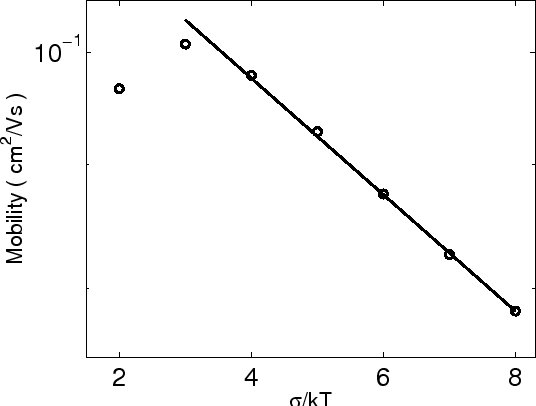
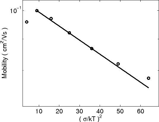
We investigated the mobility's temperature dependence in a three-dimensional hopping lattice. The crucial system parameters were set to the following values:
These results are in accordance with the measurements reorted in [79].
As the presented model expresses, only in the regime
![]() an
approximately linear relation can be observed.
an
approximately linear relation can be observed.
The mobility versus electric field characteristics predicted by the presented model is shown in
Fig 2.16. The parameters are
![]() Å,
Å, ![]() ,
,
![]() cm
cm![]() and
and
![]() .
.
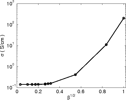
![]() , where
, where
![]() V/m, the mobility remains constant. At higher fields,
it increases with the field. Therefore,
the simple empirical relation between mobility and electric field of the
form
V/m, the mobility remains constant. At higher fields,
it increases with the field. Therefore,
the simple empirical relation between mobility and electric field of the
form
![]() is not valid for all electric fields.
is not valid for all electric fields.
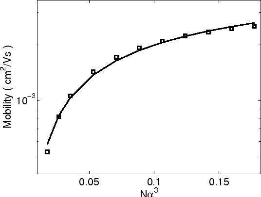
In addition to the temperature and
electric field dependence, mobility also depends on the carrier
concentration. Experiments show that
for a hole-only diode and a field effect transistor fabricated from the same
![]() -conjugated polymer, the mobility can differ up to three orders of
magnitude [79]. Empirically, the mobility's dependence on the concentration
-conjugated polymer, the mobility can differ up to three orders of
magnitude [79]. Empirically, the mobility's dependence on the concentration
![]() of localized states is written in the form
of localized states is written in the form
| (2.29) |
With the parameter
![]() Å, we compare the presented mobility
model and this empirical
formula, as shown in Fig 2.17. The agreement is quite good when we use parameters
Å, we compare the presented mobility
model and this empirical
formula, as shown in Fig 2.17. The agreement is quite good when we use parameters ![]() and
and
![]() . We notice that the value of
. We notice that the value of ![]() is different from
is different from
![]() given in [69] and
given in [69] and ![]() given in
[76]. Baranovskii [69] has stated that the parameters
given in
[76]. Baranovskii [69] has stated that the parameters
![]() and
and ![]() are temperature dependent.
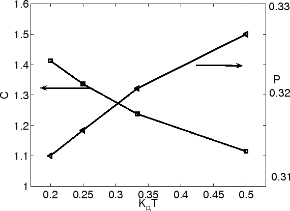
In Fig 2.18, we also show the values of parameters
are temperature dependent.
In Fig 2.18, we also show the values of parameters ![]() and
and ![]() that provide the
best fit for the solution of our model with the empirical expression (2.28). The input
parameters are
that provide the
best fit for the solution of our model with the empirical expression (2.28). The input
parameters are
![]() ,
,
![]() cm
cm![]() ,
,
![]() and
and
![]() Å. As illustrated in Fig 2.18, the parameter value of
Å. As illustrated in Fig 2.18, the parameter value of ![]() is
less than
is
less than ![]() for temperatures low enough. The value of
for temperatures low enough. The value of ![]() is decreasing with increasing temperature, a result which coincides with
[10]. Here
is decreasing with increasing temperature, a result which coincides with
[10]. Here ![]() is not constant, since the variable
range hopping (VRH)
transport mechanism is based on the interplay between the spacial and energy
factors in the exponent of transition probability, as given by (2.21). However,
assuming nearest neighbor-hopping (NNH) regime, which does not consider the effect of
energy dependent terms in (2.21) [69], leads to the values
is not constant, since the variable
range hopping (VRH)
transport mechanism is based on the interplay between the spacial and energy
factors in the exponent of transition probability, as given by (2.21). However,
assuming nearest neighbor-hopping (NNH) regime, which does not consider the effect of
energy dependent terms in (2.21) [69], leads to the values ![]() .
.
Next, we discuss the effect of the
electric field on the parameters values ![]() and
and ![]() . The results are shown
in Fig 2.19 and Fig 2.20. Input parameters are
. The results are shown
in Fig 2.19 and Fig 2.20. Input parameters are
![]() Å,
Å, ![]() kT,
kT,
![]() cm
cm![]() and
and ![]() . From these figures we can see
that the values
. From these figures we can see
that the values ![]() and
and ![]() are nearly constant in the low electric
field regime (
are nearly constant in the low electric
field regime (
![]() ).
).
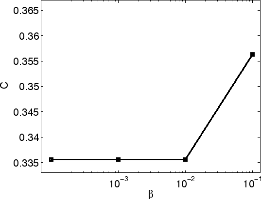
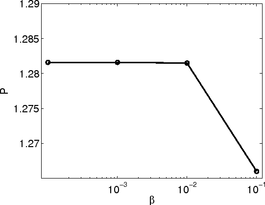
We have shown that, as expected in the variable range hopping picture, (2.24) with
![]() is only approximately valid for restricted ranges of temperature
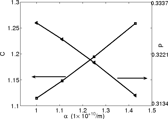
and electric field strength. So we consider the effect of the material parameter
is only approximately valid for restricted ranges of temperature
and electric field strength. So we consider the effect of the material parameter
![]() on the values of
on the values of ![]() and
and ![]() in Fig 2.21. The input parameters are
in Fig 2.21. The input parameters are
![]() ,
,
![]() and
and
![]() cm
cm![]() .
Remarkably, both parameter values
.
Remarkably, both parameter values ![]() and
and ![]() are not constant in the
given range of
are not constant in the
given range of ![]() . With increasing
. With increasing ![]() , the values of
, the values of ![]() will
decrease and the ones of
will
decrease and the ones of ![]() will increase.
will increase.