


Next: E.2 Circular Aperture
Up: E. Diffraction in Far
Previous: E. Diffraction in Far
E.1 Linear Approximation
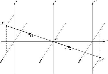
For the following discussion, Figure E.1 shows the
situation.
Figure E.1:
Standard geometry of theory of diffraction
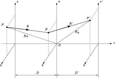 |
The aperture is positioned in the
 plane, which is normal
to the z-axis and at the position of point
plane, which is normal
to the z-axis and at the position of point  . The point source is
positioned in the
. The point source is
positioned in the  plane which is parallel to the
plane in a distance D in the negative z direction. The coordinates of the
point source are therefore
plane which is parallel to the
plane in a distance D in the negative z direction. The coordinates of the
point source are therefore  . The projection point P' with the
coordinates
. The projection point P' with the
coordinates
 is in the projection plane
  , which is parallel
to the aperture plane
also. The positions
, which is parallel
to the aperture plane
also. The positions  in
the aperture are defined by the coordinates
in
the aperture are defined by the coordinates
 . The
directions of the incoming and outgoing light waves are given with respect to
the center of the aperture plane (see
Figure E.2).
. The
directions of the incoming and outgoing light waves are given with respect to
the center of the aperture plane (see
Figure E.2).
Figure E.2:
Viewing angles of source point and projection point as seen from the
center of the aperture.
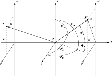 |
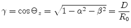
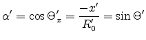
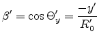
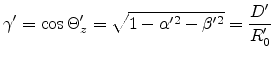
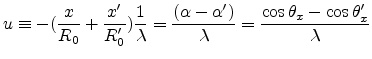
The directional vectors of the light
waves form the angles  ,
,  and
and  with their
respective axes x, y and z. Here we define the functions:
with their
respective axes x, y and z. Here we define the functions:
 |
(E.1) |
 |
(E.2) |
 |
(E.3) |
 |
(E.4) |
 |
(E.5) |
 |
(E.6) |
 |
(E.7) |
 |
(E.8) |
If one defines the transmission function:
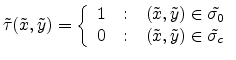 |
(E.9) |
with
 and
and
 and
and
 being the aperture area which are
transmitting and not transmitting light respectively.
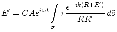
The resulting electric field on the projection side after diffraction at an aperture given by the
transmission function
being the aperture area which are
transmitting and not transmitting light respectively.
The resulting electric field on the projection side after diffraction at an aperture given by the
transmission function
 yields
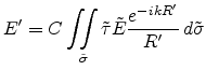 |
(E.10) |
taking the solution of a spherical wave for diffraction of a planar wave at an
infinite small aperture opening
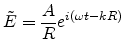 |
(E.11) |
with A as the Amplitude of the incident planar wave.
Equation (E.10) yields
 |
(E.12) |
The lengths  and
and  are given by
For the far field approximation and are linear functions of
 and
and  . Therefore we calculate the series expansion of
and around
. Therefore we calculate the series expansion of
and around  and
and  , with and given by
These distances are no functions of and . Using
(E.14) in (E.13) yields
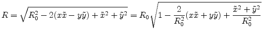 |
(E.15) |
assuming that the second and third term is much smaller than the first one,
the squareroot in (E.15) can be written as
 |
(E.16) |
and
 |
(E.17) |
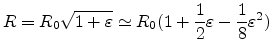
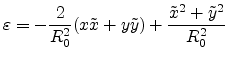
Finally R is calculated by the series expansion to the second order in
and
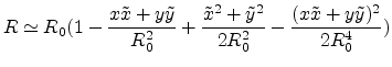 |
(E.18) |
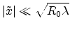
This result is only valid if
 and
and
 . This holds especially for the far field where is big in relation to
the aperture size
. This holds especially for the far field where is big in relation to
the aperture size
 |
|
 |
(E.19) |
Therefore the third term in (E.18) is
negligible and this gives
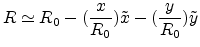 |
|
 |
(E.20) |
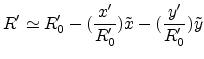
Using the approximation
 |
(E.21) |
which is valid for the far field, and the transformation of the coordinates
 |
|
 |
(E.22) |
the total optical path can be written as
 |
(E.23) |
substituting this optical path in the phase factor of the diffraction integral
in (E.12) yields
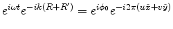 |
(E.24) |
with
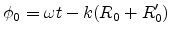 |
(E.25) |
 is not a function of and . The coordinates
 of the source and
  of the projection point are now
included in
of the projection point are now
included in  . Finally the electrical field at the projection point P'
emanating from the source point P and diffracted at the aperture with the
transmission function
. Finally the electrical field at the projection point P'
emanating from the source point P and diffracted at the aperture with the
transmission function
 can be given as
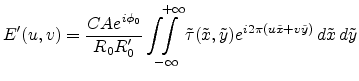 |
(E.26) |
The integral of (E.26) is exactly the
FOURIER transform of the transmission function
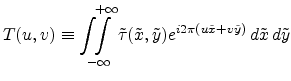 |
(E.27) |
This important result implies, that under the given assumptions, the
electrical field distribution after a diffracting aperture is proportional to
the FOURIER transform of the transmission function of the aperture.
If as shown in Figure E.3 the points
 , and
, and  are on a line, then
 and
(E.26) together with (E.27) reduces to
and
(E.26) together with (E.27) reduces to
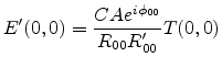 |
(E.28) |
Figure E.3:
Direct light propagation through aperture
 |
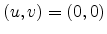
With (E.28),
(E.26) can be normalized to 
![$\displaystyle E'(u,v)=E'(0,0)\left[\frac{R_{00}R'_{00}}{R_0R'_0}\right]\frac{T(u,v)}{T(0,0)}e^{i(\phi_0-\phi_{00})}$](img552.png) |
(E.29) |
Next: E.2 Circular Aperture
Up: E. Diffraction in Far
Previous: E. Diffraction in Far
R. Minixhofer: Integrating Technology Simulation
into the Semiconductor Manufacturing Environment