Appendix C
QCL Linear Stability Analysis
The standard Maxwell-Bloch equations with a SA added can be rewritten
as [128]:
| ∂tE | = - ∂zE - ∂zE -  - - (l0 -γ|E|2)E, (l0 -γ|E|2)E, | | | (C.1) |
| ∂tP | =  DE - DE - , , | | | (C.2) |
| ∂tD | =  + +  (E*P - c.c.). (E*P - c.c.). | | | (C.3) |
The dynamics of a two-level QCL gain medium with ring cavity can be
described using the Maxwell-Bloch equations. After transformation of the
variables, the Maxwell-Bloch equations can be simplified to:
| ∂tP | = - DE - DE - , , | | | (C.5) |
To proceed with the linear stability analysis, we express each of the variables
as the sum of the steady-state value and the small perturbations δE,δP, and
δD.
The steady state solution can be found by setting the left-hand sides of the
Eqs. (C.4)-(C.6) to zero. The steady state solutions has the form E = E, P = P,
and D = D are constants in time and space satisfying:
| D | =  - - , , | | | (C.7) |
| P | =   E, E, | | | (C.8) |
| pf + 1 | =   . . | | | (C.9) |
The resulting equations regarding the fluctuations are
| ∂tδD | = -T2DE∂ER - 2EδPI - , , | | | (C.11) |
| ∂tδER | =  ![[ ( ) δE ]
- ∂zδER + δPI - l0 - 3γ ¯E2 ---R-
2](diss298x.png) , , | | | (C.12) |
| ∂tδPR | = - DδEI - DδEI - , , | | | (C.13) |
| ∂tδEI | =  ![[ ( ) δE ]
- ∂zδEI - δPR - l0 - γE¯2 ---I
2](diss302x.png) . . | | | (C.14) |
The two sets of equations, (C.10)-(C.12) and (C.13)-(C.14), are decoupled, and
translationally invariant. Thus their eigenfunctions are plane waves [126].
It holds δPI(z,t) = δPI(t)eikz, and similar for relations δD and δE
R.
The stability of the cw solution is determined by the eigenvalues of the
matrix
 | (C.15) |
If all eigenvalues have a negative real part, the cw solution is stable.
For l0 = 0 and γ = 0, the eigenvalue with the greatest real part is
λ0(K) = -ick∕n. Putting λ(K) = λ0(K) + λ1(K) into the characteristic
polynomial of M and equating the parts which are first order in l0,γ, and λ1(K),
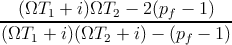
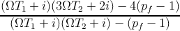
one arrives at
where pf = Dp∕Dth and Ω = kc∕n. Taking the real part of Eq. C.16 one obtains
Eq. 6.6.
 ∂zE -
∂zE - iP -
iP -
 E,
E, -
- + i
+ i .
.
![(D¯δE + δD ¯E ]
R](diss294x.png) -
- ,
,