6.3 Dynamics of QCLs
The linear stability analysis, however, predicts only the instability threshold and
does not describe the dynamics of the laser. To investigate the dynamics of QCLs
above the instability threshold, the Maxwell-Bloch equations are solved
numerically. The effect of the SA is modeled as the intensity-modulated
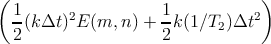
optical field amplitude in the standard Maxwell-Bloch equations [128]:
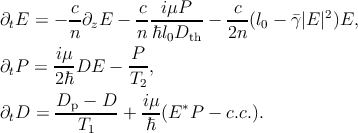 |
(6.8)
|
E and P are the envelopes of the normalized electric field and polarization,
respectively, D represents the normalized average population inversion, Dp is the
normalized steady-state population inversion, Dth is the lasing threshold value of
Dp for γ = 0, proportional to the pumping factor pf (pf ≥ 1), l0 is the linear
cavity loss, and γ = ℏ2γ∕μ2.
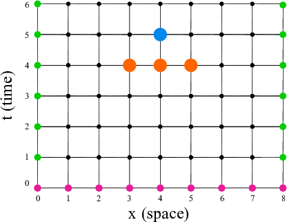
We employ a finite-difference discretization scheme to find the evolution of
electric field, polarization, and population inversion in the spatial and time
domain. A periodic boundary condition is applied to model a ring cavity. The
equations are discretized to calculate the state of the system in each step
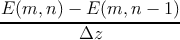
from the state in the previous step. This procedure is shown in Fig. 6.7.
The number of mesh points play an important role in preventing unreasonable
results and achieving consistency. The number should be large enough to make
sure there is not any un-inspected variation. The x - t plane is divided
into a m × n mesh points as shown in Fig. 6.7. The number of mesh
points are m = 500 and n = 105 which correspond to the grid sizes of
Δx = L∕m = 12 μm and Δt = Δx∕c = 120 fs. The periodic boundary conditions
for the dynamical variables of the QCL (electric field E, polarization P, and
population inversion D) are E(0,n) = E(L,n), P(0,n) = P(L,n), and
D(0,n) = D(L,n).
The derivatives of variables in time and space are achieved by Taylor
expansion about the grid point (m,n).
Similar expressions are written for ∂tP and ∂tD. Starting with the left hand-side
of Eq. 6.9 and 6.10 for the electric field, we have
Ė + c = = | -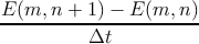 - - Δt Δt | |
|
| - + +  c2Δt2 c2Δt2 = = | |
|
|  + +  Δt Δt![[ ]
c2∂E-(m,-n)-- ∂E--(m,-n-)
∂z2 ∂t2](diss194x.png) | |
|
| = k(P - E). | (6.11) |
The expression Ė denotes ∂tE. Selecting the second equality helps to eliminate the
terms with first derivative
Solving Eq.6.12 for E(m,n + 1) gives
| E(m,n + 1) = | kΔt(P - E) | (6.13)
|
| +  Δt2 Δt2![[ ]
∂2E (m, n ) 2 ∂2E (m, n )
------2----- c -----2-----
∂t ∂x](diss199x.png) + E(m - 1,n) + E(m - 1,n) | | |
In this way, we have approximated the derivatives up to the order Δt2.
From Eq. 6.13 we have
 = Ë = k(Ṗ -Ė) - c = Ë = k(Ṗ -Ė) - c | | (6.14) |
If we multiply Eq. 6.15 by c2 and then subtract it from Eq. 6.14
 - c2 - c2 = k(Ṗ -Ė) - ck = k(Ṗ -Ė) - ck . . | | (6.16) |
As
and
Ė = k(P - E) - c , , | | |
the right side of the Eq. 6.16 can be simplified to
 | - c2 = = | |
|
| k![[ ]
(1 ∕T )(DE - P ) - k(P - E ) + c∂E--
2 ∂x](diss213x.png) + ck + ck = = | |
|
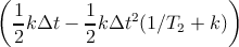
| k![[(1∕T2)(DE - P) - k(P - E)]](diss215x.png) + 2ck + 2ck - ck - ck = = | |
|
| k![[(1∕T )(DE - P) - k(P - E)]
2](diss218x.png) + 2k + 2k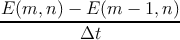 | |
|
| - k = = | |
|
| k![[(1∕T )(DE - P) - (1∕T + k)P + kE ]
2 2](diss221x.png) + 2k + 2k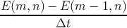 | |
|
| - k | (6.17) |
where we used the following relationship for the speed of wave propagation in
vacuum
c =  , , | | |
Therefore, evolution of electric field in time and space is given by
| E(m,n + 1) = | E(m - 1,n) + kΔt(P - E) | (6.18)
|
| +  Δt2k Δt2k![[(1∕T2)DE - (1∕T2 )P - kP + kE ]](diss226x.png) | |
|
| + kΔt[E(m,n) - E(m - 1,n)] | |
|
| - kΔt[P(m,n) - P(m - 1,n)], kΔt[P(m,n) - P(m - 1,n)], | | |
rearranging the equation results in:
| E(m,n + 1) | =  1 - kΔt 1 - kΔt E(m - 1,n) E(m - 1,n) | (6.19)
|
| +  P(m,n) P(m,n) | |
|
| +  D(m,n)E(m,n) D(m,n)E(m,n) | |
|
| +  P(m - 1,n). P(m - 1,n). | | |
Following a similar procedure, the equations for P and D are obtained. The
details and the full derivations of this method can be found in [224].
Because we have neglected noise in our treatment, the solutions would remain
|E| = |P| = 0 for all times. In order to get the laser started, one must
therefore assume a small initial disturbance of the electric field, e.g., a
Gaussian [224]
E(z, 0) = 0.1e-100( - - )2
. )2
. | | (6.20) |
The initial inversion D is set to the threshold pumping pf which is the minimum
injection current needed to start the lasing action.
| P(z, 0) = 0, D(z, 0) = pf. | | (6.21) |
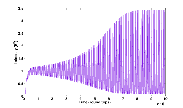
Figure 6.8 indicates the transient buildup of the intensity for a ring cavity
without the saturable absorber effect. After a few round trips, E,P, and D reach
the approximate periodic steady state. To investigate the saturable absorber
effect, we recalculate the variables including the saturable absorber term in the
Maxwell-Bloch equations, see Eq. 6.8.
For the parameters corresponding to the optimized 3QW QCL including the
SA, the lasing instability appears as the rise of the side modes with the increase of
the SA coefficient. The energy in the Rabi sidebands can change either
discontinuously or continuously at the RNGH instability threshold [126]. In
lasers with slow gain recovery time, the transition in the Rabi sidebands is
discontinuous [225], however, because of the fast gain recovery time in QCLs, Rabi
sidebands continuously grow around the central cw mode, see Fig. 6.9.
Furthermore, more Rabi side modes appear with the increase of the pumping
strength.
 -
- Δt
Δt
 +
+  Δx
Δx
 +
+  Δt
Δt![[ 2 2 ]
c2∂-E-(m,-n)-- ∂-E-(m,-n)-
∂x2 ∂t2](diss197x.png)
 =
= 
 -
-