3.5.2 Method of Moments

The basic idea behind the method of moments is not to solve the Boltzmann transport equation coupled with the Poisson equation directly, but to derive a set of balance and flux equations for macroscopic quantities based on the moments of the Boltzmann transport equation. Theoretically, an arbitrary number of equations can be derived, each containing information from the next-higher equation. As a consequence, the number of variables exceeds the number of equations. In order to obtain a closed equation system, the derivation of moments has to be truncated and a closure relation has to be formulated by a suitably chosen ansatz [81,82] based on the information incorporated in the underlying lower moments equations. Besides several theoretical approaches [83], the closure can be obtained by extraction of the missing next-higher moment from Monte-Carlo simulations [84].

In order to obtain a certain moment equation, the Boltzmann transport equation is multiplied by a general weight function and integrated over $\ensuremath{\ensuremath{\mathitbf{k}}}$ -space according to equations (3.19) and (3.20). Thereby, the series of weight functions is chosen as the powers of increasing orders of the momentum $\ensuremath {\ensuremath {\mathitbf {p}}}$ . Because of this average in $\ensuremath{\ensuremath{\mathitbf{k}}}$ -space, information on the distribution of microscopic quantities over the momentum is lost, which is originally incorporated in Boltzmann's equation. However, the information incorporated in the macroscopic equations is sufficient for a wide range of engineering applications.

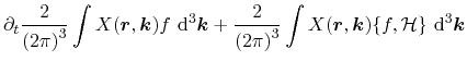
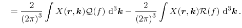
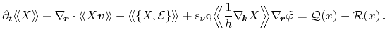
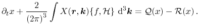
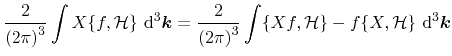
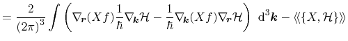
For scalar-valued weights $\ensuremath{X}$ , the application of the moment definition to Boltzmann's equation (3.10) leads to the conservation equation for the general weight function $\ensuremath{X}$

$$\ensuremath{\ensuremath{\partial_{t} \frac{2}{\left( 2 \pi \right... ...emath{f},\ensuremath{{\cal{H}}}\}} \,\, \mathrm{d}^3 \ensuremath{\mathitbf{k}}}$$ (3.25)

$$\quad= \frac{2}{\left( 2 \pi \right)^3}\ensuremath{\int \ensurema... ...{\mathcal{R}(\ensuremath{f})}} \,\, \mathrm{d}^3 \ensuremath{\mathitbf{k}}} \,.$$

which can be conveniently formulated as

$$\ensuremath{\ensuremath{\partial_{t} \ensuremath{x}}}+\frac{2}{\l... ...l{Q}(\ensuremath{x})}}-\ensuremath{\ensuremath{\mathcal{R}(\ensuremath{x})}}\,.$$ (3.26)

With the Poisson bracket identities (A.8), (A.10), and (A.11), the second term of the right hand side of equation 3.25 can be expanded as

$$\frac{2}{\left( 2 \pi \right)^3}\ensuremath{\int \ensuremath{X}\e... ...emath{X},\ensuremath{{\cal{H}}}\}} \,\, \mathrm{d}^3 \ensuremath{\mathitbf{k}}}$$ (3.27)

$$=\frac{2}{\left( 2 \pi \right)^3}\ensuremath{\int \left(\ensurema... ...ngle \ensuremath{\{\ensuremath{X},\ensuremath{{\cal{H}}}\}} \rangle \! \rangle}$$

$$=\frac{2}{\left( 2 \pi \right)^3}\int{\left(\ensuremath{\ensurema... ...remath{\ensuremath{\mathitbf{\nabla_{\!r}}}}}{\ensuremath{{\cal{H}}}}} \right)}$$

$$\quad - \ensuremath{\langle \! \langle \ensuremath{\{\ensuremath{X},\ensuremath{{\cal{H}}}\}} \rangle \! \rangle} \,.$$

Transforming the third term using Gauss' theorem and assuming $\ensuremath{f}$ to go stronger to zero than $\ensuremath{X}$ , this term vanishes [80]. Applying (3.20) to the first term, we can write the general moment equation as

$$\ensuremath{\ensuremath{\partial_{t} x}} + \ensuremath{\ensuremat... ...{Q}(\ensuremath{x})}}- \ensuremath{\ensuremath{\mathcal{R}(\ensuremath{x})}}\,.$$ (3.28)

Inserting the decomposition of the Hamilton function (3.4) into (3.28) and introducing the effective potential $\ensuremath{\tilde{\varphi}}$ , we finally obtain the macroscopic balance equation, which follows from the even, scalar-valued weight functions $\ensuremath{X}$

$$\ensuremath{\ensuremath{\partial_{t} \ensuremath{\langle \! \lang... ...{Q}(\ensuremath{x})}}- \ensuremath{\ensuremath{\mathcal{R}(\ensuremath{x})}}\,.$$ (3.29)

Analogously, formulation of the moment equation with a general odd, vector-valued weight function $\ensuremath{\ensuremath{\mathitbf{X}}}$ yields the according macroscopic flux equation

$$\ensuremath{\ensuremath{\partial_{t} \ensuremath{\langle \! \lang... ...emath{\mathcal{R}(\ensuremath{\ensuremath{\mathitbf{j}}_\ensuremath{x}})}}\ \,.$$ (3.30)

Equations (3.29) and (3.30) are the starting point for the derivation of macroscopic transport models carried out in the sequel. For homogeneous materials, $\ensuremath{\ensuremath{\ensuremath{\mathitbf{\nabla}}}}\ensuremath{\tilde{\varphi}}$ is equal to the gradient of the electrostatic potential $\ensuremath{\ensuremath{\ensuremath{\mathitbf{\nabla}}}}\ensuremath{\varphi}$ , while for inhomogeneous samples, the additional gradient of the band edges due to spatially dependent material composition enters $\ensuremath{\ensuremath{\ensuremath{\mathitbf{\nabla}}}}\ensuremath{\tilde{\varphi}}$ as well. Throughout the derivation of (3.29) and (3.30), no approximations beside the ones implied in the Boltzmann transport equation described in Section 3.2.2 were made.

M. Wagner: Simulation of Thermoelectric Devices