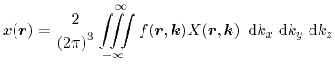
3.5.1 Microscopic and Macroscopic Quantities
While microscopic quantities represent a certain state in
 -space,
their macroscopic counterparts are averages over
-space,
their macroscopic counterparts are averages over
 -space. As a
consequence, their dependency restricts to
-space. As a
consequence, their dependency restricts to
 -space. Macroscopic
quantities are obtained by the integration of the according microscopic
quantity multiplied by the distribution function
-space. Macroscopic
quantities are obtained by the integration of the according microscopic
quantity multiplied by the distribution function
 .
The spin degeneracy is implied by a factor of two, a further factor of
.
The spin degeneracy is implied by a factor of two, a further factor of
 per degree of freedom results from the transition from discrete
states to a continuum distribution function. Thus, a general macroscopic
density
per degree of freedom results from the transition from discrete
states to a continuum distribution function. Thus, a general macroscopic
density
 reads from its microscopic, scalar-valued counterpart
 and
the distribution function
and
the distribution function
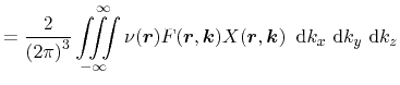
with
 as the normalized distribution function and
 the carrier
density. The short forms
the carrier
density. The short forms
 and
and
 denote the
normalized statistic average and the statistic average, respectively.
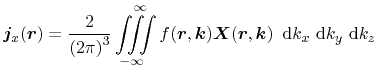
Analogously, macroscopic current densities are defined from vector-valued
microscopic quantities
denote the
normalized statistic average and the statistic average, respectively.
Analogously, macroscopic current densities are defined from vector-valued
microscopic quantities
 and the distribution function
Macroscopic densities occurring in the following derivations are the carrier
density
and the energy density
 . The corresponding fluxes are a
particle flux
. The corresponding fluxes are a
particle flux
 and the energy flux
 , respectively. The formulation
used within this work consequently implies the particle flux, which differs
from the electric current by the elementary charge. Important microscopic
quantities and their macroscopic counterparts are outlined in
Table 3.1.
, respectively. The formulation
used within this work consequently implies the particle flux, which differs
from the electric current by the elementary charge. Important microscopic
quantities and their macroscopic counterparts are outlined in
Table 3.1.
Table 3.1:
Some important macroscopic quantities for transport models with their
definition from the microscopic counterparts.
| Macroscopic quantity |
Symbol |
Definition |
| general macroscopic density |
|

|
| general macroscopic flux |

|

|
| carrier density |
|

|
| carrier flux density |
|

|
| average energy density |
|

|
| energy flux density |
|

|
|
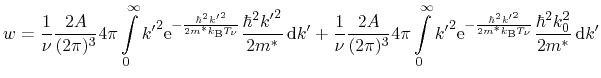
In the following, important averages are given for a heated, displaced
Maxwellian (3.17) and parabolic bands (3.13). The
carrier concentration evaluates as
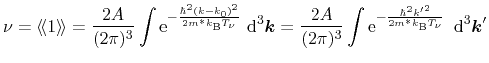 |
|
|
(3.21) |
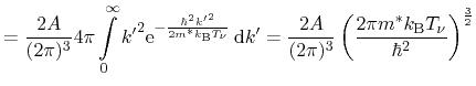 |
|
|
|
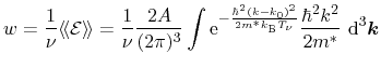
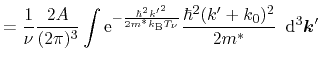
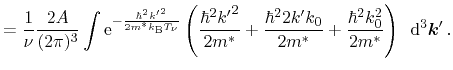
and is used to normalize further averages in the sequel. In order to derive
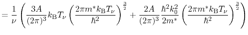
the average energy
, the average of the carrier energy
 has
to be evaluated
has
to be evaluated
The second term within the parenthesis vanishes due to the product of an odd
and an even term in the integrand. Furthermore, the transformation to polar
coordinates yields
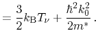
The resulting average energy consists of two parts comprising the thermal
energy by random movement and the drift energy corresponding to the average
carrier movement. For comparison, the average energy is evaluated within the
diffusion approximation, whereby the heated Maxwellian is expressed by its
first-order Taylor approximation (3.18)
In contrast to the full displaced Maxwellian, the first-order approximation
leads to a neglection of the drift component in the average energy expression.
This result underlines the range of validity of the diffusion approximation.
For a slowly drifting, hot carrier gas, the drift term in (3.23)
is negligibly small compared to the thermal energy. The formulation of the
distribution function approximation (3.18) has been
motivated exactly by this assumption.
M. Wagner: Simulation of Thermoelectric Devices