3.5.4 Relaxation Time Approximation

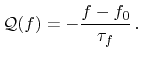
In order to obtain an expression for the right hand side of (3.29) that can be handled analytically, a commonly used simplification -- the relaxation time approximation is introduced [73]. For small deviations of the distribution function $\ensuremath{f}$ from its equilibrium state $\ensuremath{f}_0$ , the collision term can be expressed by [79]

$$\ensuremath{\ensuremath{\mathcal{Q}(\ensuremath{f})}}= - \frac{\ensuremath{f}- \ensuremath{f}_0}{\ensuremath{{\tau_{\ensuremath{f}}}}} \,.$$ (3.31)

Within this formulation, the distribution function $\ensuremath{f}$ relaxes to its equilibrium state $\ensuremath{f}_0$ with the time constant $\ensuremath{{\tau_{\ensuremath{f}}}}$ after removing all driving forces.

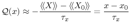
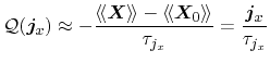
The moments of the collision term can be modeled following different strategies. Bløtekjær proposed a set of one single relaxation time for each macroscopic moment derived [88], thus the according formulations read

$$\ensuremath{\ensuremath{\mathcal{Q}(\ensuremath{x})}}\approx - \f... ...} = \frac{\ensuremath{x}- \ensuremath{x}_0}{\ensuremath{{\tau_\ensuremath{x}}}}$$ (3.32)

$$\ensuremath{\ensuremath{\mathcal{Q}(\ensuremath{\ensuremath{\math... ...suremath{\mathitbf{j}}_\ensuremath{x}}}{\ensuremath{{\tau_{j_\ensuremath{x}}}}}$$ (3.33)

for macroscopic balance and flux equations, respectively. In equilibrium, all averages of vector-valued weights vanish, thus $\ensuremath{\langle \! \langle \ensuremath{\ensuremath{\mathitbf{X}}}_0 \rangle \! \rangle} = 0$ . The relaxation times $\ensuremath{{\tau_\ensuremath{x}}}$ and $\ensuremath{{\tau_{j_\ensuremath{x}}}}$ are generally dependent on the distribution function and represent the parameters of the transport model. In order to gain accurate results, they have to be carefully calibrated. However, only the particle flux relaxation time, which is connected to the carrier mobility is accessible by measurement. Models for all other relaxation times can be extracted from Monte-Carlo simulations, which incorporate information on the full distribution function. In order to obtain a closed formulation of the transport model, the relaxation times have to be modeled with respect to quantities available in the macroscopic transport model.

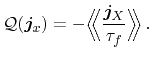
In contrast to the macroscopic relaxation time approximation applied in Bløtekjær's approach, Stratton's ansatz incorporates one microscopic relaxation time $\ensuremath{{\tau}}$ for the entire transport model that describes the scattering of single carriers. Therefrom, the according formulation for the collision term reads

$$\ensuremath{\ensuremath{\mathcal{Q}(\ensuremath{\ensuremath{\math... ...h{X}}}{\ensuremath{{\tau}}_\ensuremath{f}} \Bigr\rangle \! \! \Bigr\rangle} \,.$$ (3.34)

The weights for the odd moment equations are chosen in a way that the right sides become the fluxes themselves. As a consequence, additional terms in the flux equations appear, which are systematically derived and analyzed in the sequel. The relaxation time $\ensuremath{{\tau}}$ is often modeled to depend on the energy by a power law

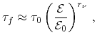$$\ensuremath{{\tau}}_\ensuremath{f}\approx \ensuremath{\tau_0}\lef... ...th{\mathcal{E}}}{\ensuremath{\mathcal{E}}_0} \right)^{{\ensuremath{r_\nu}}} \,,$$ (3.35)

which enables the analytical treatment of several integrals. Depending on the dominant scattering mechanism, the scattering parameter ${\ensuremath{r_\nu}}$ takes values between $-1/2$ for acoustic phonon scattering and $3/2$ for ionized impurity scattering. While expression (3.35) is valid with a constant $\ensuremath{\tau_0}$ for acoustic phonon scattering, $\ensuremath{\tau_0}$ is slightly energy dependent for ionized impurity scattering [73].

M. Wagner: Simulation of Thermoelectric Devices