3.5.8 Summary of Equations

In the following, the equations derived applying both Stratton's and Bløtekjær's approach are summarized. While the balance equations, which belong to scalar weights are equivalent for both approaches, the flux equations differ due to the different approaches of relaxation time approximations to the collision term as well as the associated choice of weights. For both Stratton's and Bløtekjær's approach the carrier balance equation and energy balance equation read

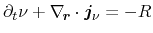$$\ensuremath{\ensuremath{\partial_{t} \ensuremath{\nu}}} + \ensure... ...\ensuremath{\cdot}}\ensuremath{\ensuremath{\mathitbf{j}}_\nu}= - \ensuremath{R}$$ (3.111)

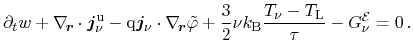$$\ensuremath{\ensuremath{\partial_{t} \ensuremath{w}}} + \ensurema... ...math{T_{\mathrm{L}}}}{\tau} - \ensuremath{G_\nu^\ensuremath{\mathcal{E}}}= 0\,.$$ (3.112)

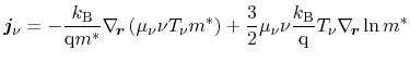
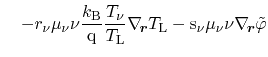
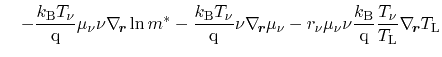
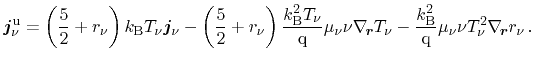
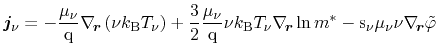
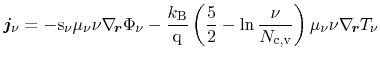
The carrier flux and energy flux equations derived by using Stratton's microscopic relaxation time ansatz are

$$\ensuremath{\ensuremath{\mathitbf{j}}_\nu}= - \frac{k_\ensuremath... ...math{\nu}}\ensuremath{\ensuremath{\ensuremath{\mathitbf{\nabla_{\!r}}}}}\ln m^*$$ (3.113)

$$\quad - {\ensuremath{r_\nu}}\ensuremath{\ensuremath{\mu}_\nu}\ens... ...{\ensuremath{\ensuremath{\mathitbf{\nabla_{\!r}}}}}\ensuremath{\tilde{\varphi}}$$

$$\ensuremath{\ensuremath{\mathitbf{j}}_\nu^\mathrm{u}}= - \frac{k_... ...h{\nu}}^2 \ensuremath{\ensuremath{\ensuremath{\mathitbf{\nabla_{\!r}}}}}\ln m^*$$ (3.114)

$$\quad - \left( {\ensuremath{r_\nu}}+ \frac{5}{2} \right) {\ensure... ...suremath{\ensuremath{\mathitbf{\nabla_{\!r}}}}} \ensuremath{\tilde{\varphi}}\,.$$

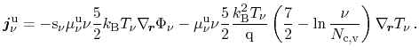
The according formulation with the electrochemical potential introduced reads

$$\ensuremath{\ensuremath{\mathitbf{j}}_\nu}= - \ensuremath{\mathrm... ...nsuremath{\ensuremath{\mathitbf{\nabla_{\!r}}}}}\ensuremath{T_\ensuremath{\nu}}$$ (3.115)

$$\quad - \frac{k_\ensuremath{\mathrm{B}}\ensuremath{T_\ensuremath{... ...h{\ensuremath{\ensuremath{\mathitbf{\nabla_{\!r}}}}}\ensuremath{T_{\mathrm{L}}}$$

$$\ensuremath{\ensuremath{\mathitbf{j}}_\nu^\mathrm{u}}= - \ensurem... ...nsuremath{\ensuremath{\mathitbf{\nabla_{\!r}}}}}\ensuremath{T_\ensuremath{\nu}}$$ (3.116)

$$\quad - \frac{k_\ensuremath{\mathrm{B}}^2}{\mathrm{q}} \ensuremat... ...h{\nu}}^2 \ensuremath{\ensuremath{\ensuremath{\mathitbf{\nabla_{\!r}}}}}\ln m^*$$

$$\quad - {\ensuremath{r_\nu}}\frac{k_\ensuremath{\mathrm{B}}^2 \en... ...ensuremath{\ensuremath{\mathitbf{\nabla_{\!r}}}}}\ensuremath{T_{\mathrm{L}}}\,.$$

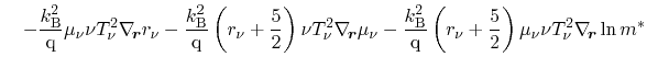
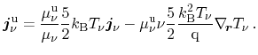
In some cases, it is convenient to formulate the energy flux in terms of the particle flux. For Stratton's equations, it is given by

$$\ensuremath{\ensuremath{\mathitbf{j}}_\nu^\mathrm{u}}= \left( \fr... ...emath{\ensuremath{\ensuremath{\mathitbf{\nabla_{\!r}}}}}{\ensuremath{r_\nu}}\,.$$ (3.117)

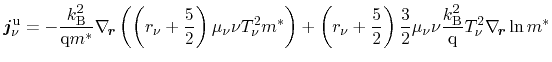
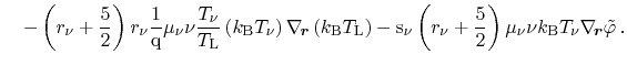
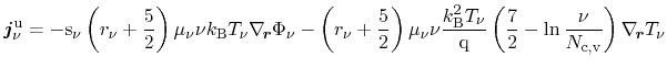
Bløtekjær's concept of macroscopic relaxation times yields for the particle and energy flux equations, respectively

$$\ensuremath{\ensuremath{\mathitbf{j}}_\nu}= - \frac{\ensuremath{\... ...{\ensuremath{\ensuremath{\mathitbf{\nabla_{\!r}}}}}\ensuremath{\tilde{\varphi}}$$ (3.118)

$$\ensuremath{\ensuremath{\mathitbf{j}}_\nu^\mathrm{u}}= - \frac{5}... ...nsuremath{\ensuremath{\mathitbf{\nabla_{\!r}}}}}\ensuremath{\tilde{\varphi}}\,.$$ (3.119)

With the electrochemical potential, they are

$$\ensuremath{\ensuremath{\mathitbf{j}}_\nu}= - \ensuremath{\mathrm... ...nsuremath{\ensuremath{\mathitbf{\nabla_{\!r}}}}}\ensuremath{T_\ensuremath{\nu}}$$ (3.120)

$$\ensuremath{\ensuremath{\mathitbf{j}}_\nu^\mathrm{u}}= - \ensurem... ...emath{\ensuremath{\mathitbf{\nabla_{\!r}}}}} \ensuremath{T_\ensuremath{\nu}}\,.$$ (3.121)

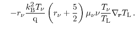
Formulation of the energy flux in terms of the particle flux yields

$$\ensuremath{\ensuremath{\mathitbf{j}}_\nu^\mathrm{u}}= \frac{\ens... ...remath{\ensuremath{\mathitbf{\nabla_{\!r}}}}}\ensuremath{T_\ensuremath{\nu}}\,.$$ (3.122)

Compared to Bløtekjær's model, Stratton's equations incorporate additional gradients of the mobility and the lattice temperature resulting from the formulation of the microscopic relaxation time in a power-law. The exponent ${\ensuremath{r_\nu}}$ enters the equations as a further model parameter, which has to be approximated to account for the dominant scattering mechanisms. It depends on both the doping profile and the temperature and can be in the range $\left[-0.5,1.5\right]$ [73]. Generally, both approaches are able to cover the physical background on the same level [92]. However, it has to be kept in mind that the definitions of the mobilities employed in both model equations differ significantly. In the homogeneous case, the mobilities are equal [92,93], but for locally changing driving forces, they diverge. While the mobility in Bløtekjær's equations can be approximated by the energy dependent bulk value, the definition in Stratton's model is always different [86]. Thus, for engineering purposes, transport description based on Bløtekjær's equations is more convenient.

M. Wagner: Simulation of Thermoelectric Devices