3.5.9 Onsager Relations
The relationship between Seebeck and Peltier coefficient has been
identified in the pioneering work by Kelvin and formulated in the first
Kelvin relation. However, Onsager formulated an extended theory valid
for general systems consisting of several mutually dependent irreversible
processes [12]. His theory is based on thermodynamics and the
general principle of time symmetry and holds for systems around their
equilibrium. Every flux of a certain quantity  within a system is given
by the linear combination of according driving forces
within a system is given
by the linear combination of according driving forces
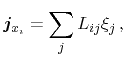 |
(3.123) |
while each flux has an assigned driving force defined by the derivative of the
system's entropy with respect to the according quantity [94]
 |
(3.124) |
Following (3.123), the affinities
 describe the
deviation from equilibrium, which is characterized by zero currents. In
equilibrium, the entropy
describe the
deviation from equilibrium, which is characterized by zero currents. In
equilibrium, the entropy  reaches a maximum. Onsager's reciprocal
relations state the identities of the cross coefficients
reaches a maximum. Onsager's reciprocal
relations state the identities of the cross coefficients
 |
(3.125) |
for vanishing magnetic fields. The cross coefficients  are a measure
for the coupling of the single transport phenomena within the system. A system
with
are a measure
for the coupling of the single transport phenomena within the system. A system
with  consists of independent irreversible processes, where every
driving force only affects its connected flux. A convenient form to identify
the according affinities to given fluxes is obtained by considering the time
derivative of the entropy
consists of independent irreversible processes, where every
driving force only affects its connected flux. A convenient form to identify
the according affinities to given fluxes is obtained by considering the time
derivative of the entropy
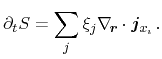 |
(3.126) |
For the thermoelectric case, the basic relations are given from irreversible
thermodynamics [9]. In local thermodynamic equilibrium, the
differential total energy is obtained as the sum of products of corresponding
internal variable and the differential external variable
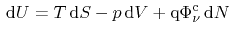 |
(3.127) |
with the number of particles within the system  and the chemical potential
 , which is the difference of the electrochemical and electrostatic
potentials. Since the electrostatic potential is connected to the carrier
densities as well as doping densities by Poisson's equation, it is not an
independent variable in the thermodynamic sense. Neglecting thermal expansion,
the
, which is the difference of the electrochemical and electrostatic
potentials. Since the electrostatic potential is connected to the carrier
densities as well as doping densities by Poisson's equation, it is not an
independent variable in the thermodynamic sense. Neglecting thermal expansion,
the  -term vanishes. Thus, expression of the differential entropy
results in
-term vanishes. Thus, expression of the differential entropy
results in
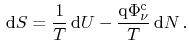 |
(3.128) |
Introducing the according current densities, the entropy flux becomes
 |
(3.129) |
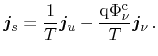
Formulating balance equations for the entropy, the total energy, and the
particle density, as well as assuming steady state conditions, the change of
entropy for the thermoelectric case is obtained as
 |
(3.130) |
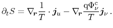
According to the definition of heat
 , the heat flux equation can
be obtained from the energy flux as
, the heat flux equation can
be obtained from the energy flux as
 |
(3.131) |
Thus, the change of entropy with respect to the heat flux instead of the total
energy flux reads
 |
(3.132) |
From (3.130), it follows that if particle current and total energy
current are considered as fluxes, the according affinities are
 and
and
 . A more convenient choice can be extracted from
(3.132), where the affinities
and
. A more convenient choice can be extracted from
(3.132), where the affinities
and
 follow from the particle current and the heat current as chosen fluxes.
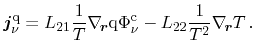
In the sequel, the combination of particle flux and heat flux has been chosen
for the analysis of several transport models derived. The general equations
for particle and heat flux with the Onsager coefficients
read
follow from the particle current and the heat current as chosen fluxes.
In the sequel, the combination of particle flux and heat flux has been chosen
for the analysis of several transport models derived. The general equations
for particle and heat flux with the Onsager coefficients
read
 |
|
|
(3.133) |
 |
|
|
(3.134) |
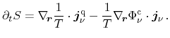
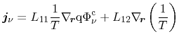
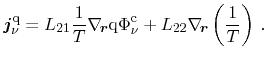
The expansion of the temperature derivatives results in a more convenient form
which can be used for a direct coefficient comparison with the transport
equations obtained previously
 |
|
|
(3.135) |
 |
|
|
(3.136) |
Particle current and heat current obtained by Bløtekjær's approach read
A coefficient comparison between (3.135) and (3.137) as
well as (3.136) and (3.139) yields the Onsager
coefficients
 |
|
|
(3.139) |
 |
|
|
(3.140) |
As a consequence of the macroscopic relaxation time approximation, where one
relaxation time for every current is introduced, different mobility definitions
enter the particle current and heat current. Thus, the model obtained by
Bløtekjær's approach does not inherently fulfill Onsager's reciprocity theorem.
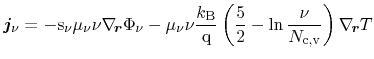
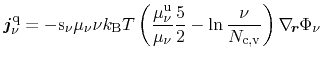
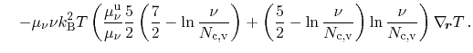
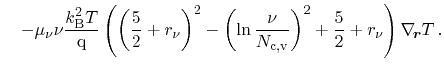
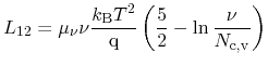
Next, the model obtained by Stratton's approach is analyzed. The equations
for particle and heat flux are obtained for homogeneous materials as
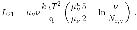
Analogously, the Onsager coefficients are identified by a coefficient
comparison between (3.135) and (3.141) as well as
(3.136) and (3.142) as
 |
(3.143) |
For the Stratton model, Onsager's reciprocity theorem holds due to the
application of the microscopic relaxation time approximation, where a single
relaxation time enters all fluxes.
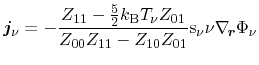
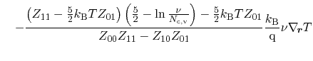
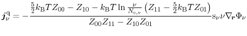
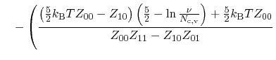
Finally, the model derived in Section 3.5.7 is analyzed. In contrast to
the other models, the stochastic part is described by a linear combination of
all fluxes taken into account. The final particle current and heat current
equations are
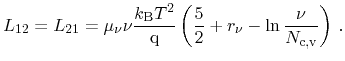
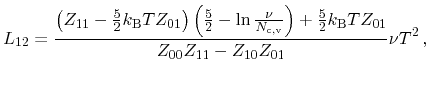
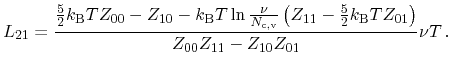
The Onsager coefficients are identified in the usual way by a coefficient
comparison between (3.135) and (3.145) as well as
(3.136) and (3.146), respectively. Thus, the according Onsager
coefficients are
 |
|
|
(3.146) |
 |
|
|
(3.147) |
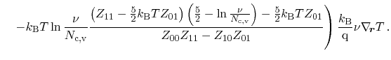
A comparison of the relevant parameters results in the relation
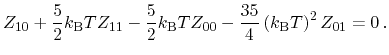 |
(3.148) |
Briefly summarized, Stratton's equations inherently fulfill the Onsager
relations, while the Onsager conformity of Bløtekjær's equations depends on the
choice of the model parameters. This is a consequence of the extended degrees
of freedom due to the additional model parameters introduced by the macroscopic
relaxation time approximation. For the non-diagonal ansatz, the reciprocity
principle is fulfilled, when the model is parametrized obeying the relation
(3.148).
M. Wagner: Simulation of Thermoelectric Devices