C.1 The Neumann Boundary for the Rotor-Rotor-Operator

The Neumann boundary integral (5.29) becomes

$$\int_{\mathcal{A}_{N1}}\vec{n}\cdot\left[ \vec{N}_i\times\left( \... ...{1}{\gamma}\vec{\nabla}\times\vec{N}_j \right) \right] \mathrm{d}A = [D]\{c\}.$$ (C.1)

The assembly of the matrix $[D]$ with entries

$$D_{ij} = \int_{\mathcal{A}_{N1}}\vec{n}\cdot\left[ \vec{N}_i\times\left( \frac{1}{\gamma}\vec{\nabla}\times\vec{N}_j \right) \right] \mathrm{d}A$$ (C.2)

is performed element by element, whereby only the elements lying on the Neumann boundary are considered. The elements are tetrahedra and in each element $\vec{N}_i$ is represented by the vector edge functions (5.45) to (5.50).

The integral domain transformation for an arbitrary surface in the three-dimensional space is the same as in Appendix A and is derived in a similar manner. The integral is represented as a sum

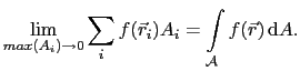$$\lim_{max(A_i)\rightarrow{}0}\sum_if(\vec{r}_i)A_i = \int_{\mathcal{A}}f(\vec{r}) \mathrm{d}A.$$ (C.3)

The surface $\mathcal{A}$ is subdivided into pieces $\mathcal{A}_i$ with areas $A_i$ . $\vec{r}_i$ is point inside $\mathcal{A}_i$ . The transformation is given by

$$\vec{r} = \vec{r}\left(x(\xi,\eta), y(\xi,\eta), z(\xi,\eta)\right).$$ (C.4)

An area $A_i$ is calculated as

$$\begin{split}A_i & = \left\vert [\vec{r}(\xi+h,\eta) - \vec{r... ...\times\vec{r}_{\eta}(\xi,\eta)\right]hk\right\vert, \end{split}$$ (C.5)

which leads again to (A.8) and (A.7).

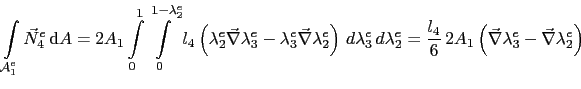
Now the element matrix $[D]^e$ can be computed. As there are four outer triangular faces on each tetrahedral element, there will be four different element matrices for each face which lies on the Neumann boundary

$$\begin{split}D_{ij}^e & = \int_{\mathcal{A}^e_k}\vec{n}_k\cdo... ...ma}\vec{\nabla}\times\vec{N}^e_j\right), k\in[1;4] \end{split}$$ (C.6)

and using (5.52)

$$D_{ij}^e = \frac{1}{3\gamma V_e}\left(\vec{n}_k\times\int_{\math... ...ec{N}^e_i \mathrm{d}A\right)\cdot\left(l_j \vec{r}_{7-j}\right), k\in[1;4].$$ (C.7)

$\mathcal{A}^e_k$ is the face opposite to the node $k$ . $\vec{n}_k$ is a constant vector with the characteristic length 1, perpendicular to $\mathcal{A}^e_k$ and points outwards. $\gamma$ is assumed to be constant in each element. Only the three $\vec{N}^e_i$ functions for the edges in the $\mathcal{A}^e_k$ plane are not perpendicular to $A^e_k$ . The remaining three vector functions are perpendicular to $A^e_k$ . Consequently these vectors are parallel to $\vec{n}_k$ and the corresponding vector product $\vec{n}_k\times\vec{N}^e_i$ becomes zero.

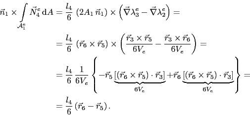
For the element face $\mathcal{A}^e_1$ the element matrix is given as follows

$$D_{1j}^e = D_{2j}^e = D_{3j}^e = 0$$ (C.8)

$$D_{4j}^e = \frac{1}{3\gamma V_e}\left(\vec{n}_1\times\int_{\math... ...ec{N}^e_4 \mathrm{d}A\right)\cdot\left(l_j \vec{r}_{7-j}\right), k\in[1;4].$$ (C.9)

The integral is computed using the integral domain transformation discussed above.

$$\int_{\mathcal{A}^e_1}\vec{N}^e_4 \mathrm{d}A = 2A_1\int_0^1\int... ...rac{l_4}{6} 2A_1\left(\vec{\nabla}\lambda^e_3 - \vec{\nabla}\lambda^e_2\right)$$ (C.10)

$$\begin{split}\vec{n}_1\times\int_{\mathcal{A}^e_1}\vec{N}^e_4... ... = \frac{l_4}{6}\left(\vec{r}_6 - \vec{r}_5\right). \end{split}$$ (C.11)

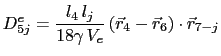
Thus the final solution for the fourth edge ($i=4$ ) is given by the expression

$$D_{4j}^e = \frac{l_4 l_j}{18\gamma V_e}\left(\vec{r}_6 - \vec{r}_5\right)\cdot\vec{r}_{7-j}.$$ (C.12)

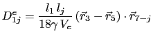
The same procedure is used for remaining edges (with index $i$ ):

$$D_{5j}^e = \frac{l_4 l_j}{18\gamma V_e}\left(\vec{r}_4 - \vec{r}_6\right)\cdot\vec{r}_{7-j}$$ (C.13)

$$D_{6j}^e = \frac{l_4 l_j}{18\gamma V_e}\left(\vec{r}_5 - \vec{r}_4\right)\cdot\vec{r}_{7-j}.$$ (C.14)

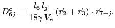
Analogously it is proceeded for the remaining faces.

For the face $\mathcal{A}^e_2$ :

$$D_{1j}^e = D_{4j}^e = D_{5j}^e = 0$$ (C.15)

$$D_{2j}^e = -\frac{l_2 l_j}{18\gamma V_e}\left(\vec{r}_6 + \vec{r}_3\right)\cdot\vec{r}_{7-j}$$ (C.16)

$$D_{3j}^e = \frac{l_3 l_j}{18\gamma V_e}\left(\vec{r}_2 - \vec{r}_6\right)\cdot\vec{r}_{7-j}$$ (C.17)

$$D_{6j}^e = \frac{l_6 l_j}{18\gamma V_e}\left(\vec{r}_2 + \vec{r}_3\right)\cdot\vec{r}_{7-j}.$$ (C.18)

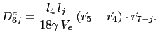
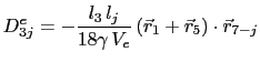
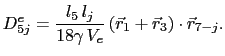
For the face $\mathcal{A}^e_3$ :

$$D_{2j}^e = D_{4j}^e = D_{6j}^e = 0$$ (C.19)

$$D_{1j}^e = \frac{l_1 l_j}{18\gamma V_e}\left(\vec{r}_3 - \vec{r}_5\right)\cdot\vec{r}_{7-j}$$ (C.20)

$$D_{3j}^e = -\frac{l_3 l_j}{18\gamma V_e}\left(\vec{r}_1 + \vec{r}_5\right)\cdot\vec{r}_{7-j}$$ (C.21)

$$D_{5j}^e = \frac{l_5 l_j}{18\gamma V_e}\left(\vec{r}_1 + \vec{r}_3\right)\cdot\vec{r}_{7-j}.$$ (C.22)

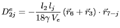
For the face $\mathcal{A}^e_4$ :

$$D_{3j}^e = D_{5j}^e = D_{6j}^e = 0$$ (C.23)

$$D_{1j}^e = -\frac{l_1 l_j}{18\gamma V_e}\left(\vec{r}_2 + \vec{r}_4\right)\cdot\vec{r}_{7-j}$$ (C.24)

$$D_{2j}^e = \frac{l_2 l_j}{18\gamma V_e}\left(\vec{r}_1 - \vec{r}_4\right)\cdot\vec{r}_{7-j}$$ (C.25)

$$D_{4j}^e = \frac{l_4 l_j}{18\gamma V_e}\left(\vec{r}_1 + \vec{r}_2\right)\cdot\vec{r}_{7-j}.$$ (C.26)