3.1 Electro-Thermal Problem

Denoting the electric potential at any point in the line by $\symElecPot$ and the electrical conductivity by $\symElecCond$, the current density can be calculated from Ohm's law as

$$\vec\symCurrDens=\symElecCond\vec\symElecField = -\symElecCond\ensuremath{\nabla{\symElecPot}},$$ (3.1)

where the electric field is related to the electric potential by

$$\vec\symElecField = -\ensuremath{\nabla{\symElecPot}}.$$ (3.2)

Since the electric charge should obviously be conserved, one can write

$$\ensuremath{\nabla\cdot{\vec\symCurrDens}} = 0,$$ (3.3)

which together with (3.1) yields an equation written for the electric potential,

$$\ensuremath{\nabla\cdot{(\symElecCond\ensuremath{\nabla{\symElecPot}})}} = 0.$$ (3.4)

Note that (3.4) reduces to the Laplace equation,

$$\ensuremath{\nabla^2 \symElecPot} = 0,$$ (3.5)

if the electrical conductivity is constant along the line.

The temperature distribution is determined by the solution of the thermal problem

$$\ensuremath{\nabla\cdot{(\symThermCond\ensuremath{\nabla{T}})}} =... ...ecHeat\ensuremath{\ensuremath{\frac{\partial \T}{\partial t}}} - \symElecPower,$$ (3.6)

where $\symThermCond$ is the material thermal conductivity, $\symMatDens$ is the mass density, and $\symSpecHeat$ is the specific heat. Here, $\symElecPower$ is the electrical power loss density, given by

$$\symElecPower = \symElecCond\symElecField^2 = \symElecCond\left(\ensuremath{\nabla{\symElecPot}}\right)^2,$$ (3.7)

which accounts for the Joule heating and couples the electrical with the thermal problem.

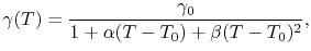
Both, the electrical and thermal conductivity are treated as temperature dependent parameters, following the form

$$\gamma(\T) = \frac{\symRefCond}{1+\symLinTempCoef(\T-\TO)+\symQuadTempCoef(\T-\TO)^2},$$ (3.8)

where $\symRefCond$ is the conductivity for a given reference temperature $\TO$. Here, $\symLinTempCoef$ and $\symQuadTempCoef$ are the linear and quadratic temperature coefficients, respectively.

The equations (3.4) and (3.6), together with (3.7) and (3.8), compose a non-linear system of equations, whose solution provides the voltage, electric field, current density, and temperature distributions in an interconnect line. It should be pointed out that special attention must be taken in setting the thermal boundary conditions. In order to properly consider the effect of Joule heating, a sufficient big portion of dielectric surrounding must be included in the simulation. A thermal reservoir can be implemented by a Dirichlet boundary condition for the temperature.