3.6 Model Summary

The developed electromigration model consists of several submodels. The electrical and temperature distribution in the interconnect is determined by the system of equations

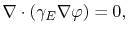$$\ensuremath{\nabla\cdot{(\symElecCond\ensuremath{\nabla{\symElecPot}})}} = 0,$$ (3.71)

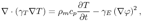$$\ensuremath{\nabla\cdot{(\symThermCond\ensuremath{\nabla{T}})}} =... ...T}{\partial t}}} - \symElecCond\left(\ensuremath{\nabla{\symElecPot}}\right)^2,$$ (3.72)

with temperature dependent conductivities

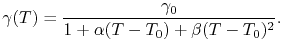$$\gamma(\T) = \frac{\symRefCond}{1+\symLinTempCoef(\T-\TO)+\symQuadTempCoef(\T-\TO)^2}.$$ (3.73)

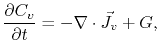
The vacancy flux is given by

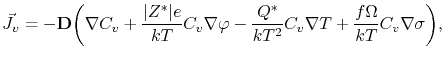$$\vec\JV = -\mathbf{D} \biggl(\ensuremath{\nabla{\CV}} + \frac{\ve... ...symVacRelFactor\symAtomVol}{\kB\T}\CV\ensuremath{\nabla{\symHydStress}}\biggr),$$ (3.74)

which takes into account all driving forces for vacancy transport. The vacancy dynamics is then described by the equations

$$\ensuremath{\ensuremath{\frac{\partial \CV}{\partial t}}}= -\ensuremath{\nabla\cdot{\vec\JV}} + \G,% = -\Div{\vec\JV} + \Dert{\Cim},$$ (3.75)

$$\G = \ensuremath{\ensuremath{\frac{\partial \Cim}{\partial t}}}= ... ...R}{\symOmT\CV}\right)\right] = \frac{1}{\symVacRelTime}\left(\Ceq-q\Cim\right),$$ (3.76)

where the latter is calculated at grain boundaries and interfaces only.

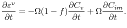
The trace of the total electromigration strain is calculated by

$$\ensuremath{\ensuremath{\frac{\partial \symStrain^{v}}{\partial t... ...\symVacRelFactor)\ensuremath{\nabla\cdot{\vec\JV}} + \symVacRelFactor\G\right],$$ (3.77)

which together with (3.75) and (3.76) can be conveniently expressed as

$$\ensuremath{\ensuremath{\frac{\partial \symStrain^{v}}{\partial t... ...l t}}} + \symAtomVol\ensuremath{\ensuremath{\frac{\partial \Cim}{\partial t}}}.$$ (3.78)

The resultant line deformation and mechanical stress is determined by the set of equations

$$\boldsymbol\symStrain = \mathbf{S}\mathbf{u},$$ (3.79)

$$\ensuremath{\nabla\cdot{\boldsymbol\symHydStress}} = 0,$$ (3.80)

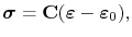$$\boldsymbol\symHydStress = \mathbf{C}(\boldsymbol\symStrain - \boldsymbol\symStrain_{0}),$$ (3.81)

where

$$\boldsymbol\symStrain_{0} = \frac{1}{3}\symStrain^v\mathbf{I}.$$ (3.82)

The solution of these equations allows a complete cycle of simulation of electromigration in general three-dimensional interconnet structures.