The surface roughness induced spin relaxation matrix elements are calculated between wave functions with opposite spin projections. The matrix elements are calculated in the same manner as in Chapter 6, i.e. the spin relaxation matrix elements normalized to the value of the intrasubband scattering at zero strain are written as
|
| (7.1) |
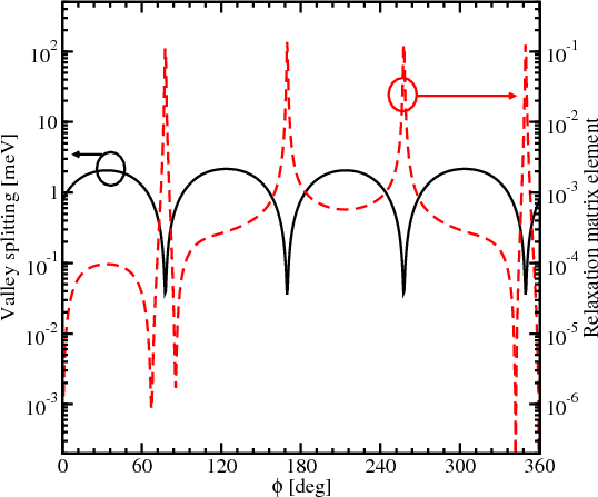
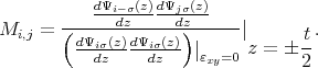
Figure 7.1 and Figure 7.2 show the spin relaxation matrix elements (normalized to intravalley scattering at zero strain)
on the angle between the incident and scattered wave vectors together with the valley splitting for the scattered wave.
Oscillations of the valley splitting are observed. In Figure 7.1 the sharp increase of the relaxation matrix element is
correlated with the reduction of the valley splitting which occurs for the values of the angle determined by zeroes of the
Dεxy - term. This is the condition of the formation of the so called spin hot spots characterized by the maximum spin
mixing. In contrast to Figure 7.1, the valley splitting reduction due to the
term. This is the condition of the formation of the so called spin hot spots characterized by the maximum spin
mixing. In contrast to Figure 7.1, the valley splitting reduction due to the  term shown in Figure 7.2
does not lead to a sharp increase of the spin relaxation matrix elements on the angle between the incident and scattered
waves.
term shown in Figure 7.2
does not lead to a sharp increase of the spin relaxation matrix elements on the angle between the incident and scattered
waves.
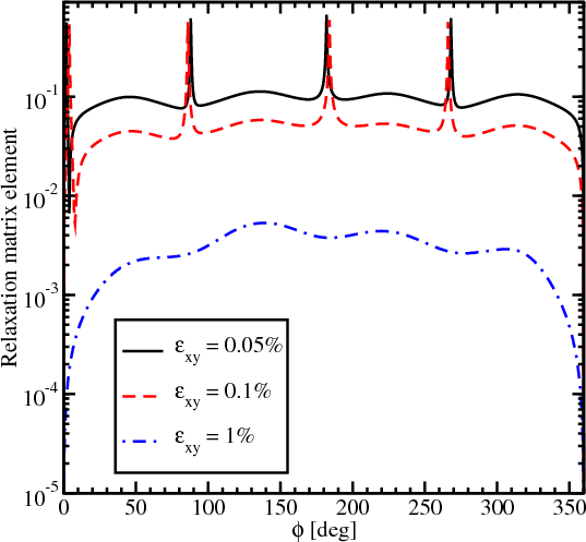
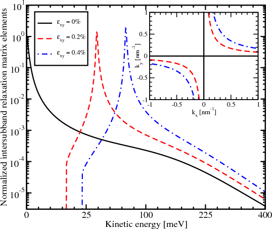
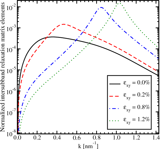
The splitting between the subbands depends on Dεxy - kxky∕M and their degeneracy is lifted by the kinetic-like term kxky∕M even without shear strain. This results in a strong dependence of the surface roughness induced spin relaxation matrix elements on the angle between the incident and outgoing wave vectors (Figure 7.1 and Figure 7.2). Figure 7.3 shows the dependences of the relaxation matrix elements on this angle for different values of shear strain. The sharp peaks in Figure 7.3 for shear strain values 0.05% and 0.1% nature of which were discussed for Figure 7.1 and Figure 7.2 are observed for similar angle values. However, the intersubband matrix relaxation elements for higher strain show lower values, except peaks. For the shear strain of 1% no peaks are observed and the matrix element values are smaller by several orders of magnitude. As follows from Figure 7.3, shear strain leads to the reduction of the spin relaxation matrix element.
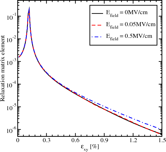
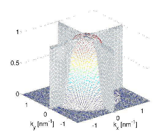
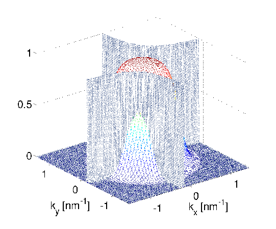
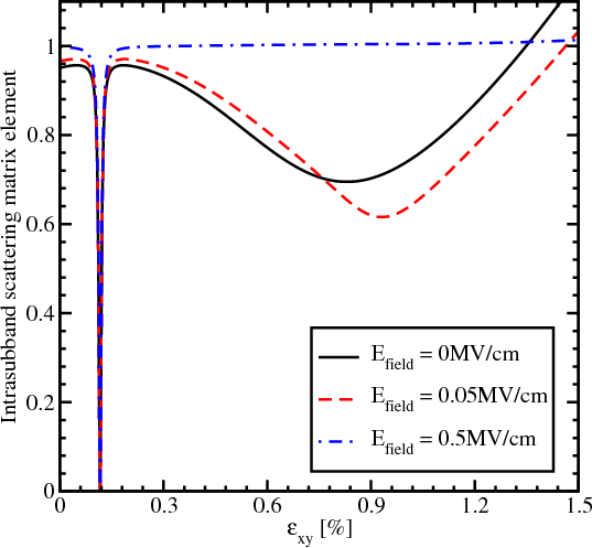
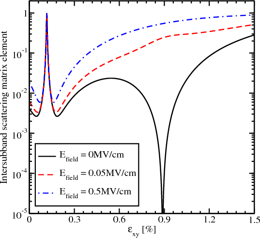
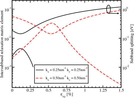
Figure 7.4 and Figure 7.5 show the dependences on strain and electric field of the matrix elements for the intrasubband
and intersubband scattering. The intrasubband scattering matrix elements have two decreasing regions shown in Figure 7.4.
These regions are in good agreement with the valley splitting minima in Figure 5.19. For higher fields the second decreasing
region around the shear strain value of 0.931% vanishes. For the electric field of 0.5MV/cm the intrasubband matrix
elements are sharply reduced only for the shear strain value of 0.116%. At the same time, the intersubband matrix elements
show a sharp increase around the shear strain value of 0.116%. The electric field does not affect much the valley splitting
provided by the zero value of the term Dεxy - , and the sharp increase in the intersubband matrix elements is
observed at higher fields. At the same time the electric field washes out a sharp minimum around the shear
strain value of 0.931% in Figure 7.5. With the electric field increased the confinement pushes the carriers
closer to the interface which results in both an intersubband and an intrasubband scattering matrix elements
increase.
, and the sharp increase in the intersubband matrix elements is
observed at higher fields. At the same time the electric field washes out a sharp minimum around the shear
strain value of 0.931% in Figure 7.5. With the electric field increased the confinement pushes the carriers
closer to the interface which results in both an intersubband and an intrasubband scattering matrix elements
increase.
The dependence of the spin relaxation matrix elements on shear strain for several values of the electric field is shown in Figure 7.6. The spin relaxation matrix elements increase until the strain value 0.116%, the point determined by the spin hot spot condition. Applying strain larger than 0.116% suppresses the spin relaxation significantly, for all values of the electric field. In contrary to the scattering matrix elements (Figure 7.4 and Figure 7.5), the relaxation matrix elements demonstrate a sharp feature only for the shear strain value of 0.116% at zero electric field. Large electric field leads to an increase of the relaxation matrix elements due to the additional field-induced confinement resulting in higher values of the surface roughness induced spin relaxation matrix elements.
Figure 7.7 displays the normalized spin relaxation matrix elements for an unstrained film. The "hot spots" are along the [100] and [010] directions. Shear strain pushes the "hot spots" to higher energies (Figure 7.8) outside of the states occupied by carriers. This leads to a reduction of the spin relaxation.
The surface roughness spin relaxation rate is calculated in the following way [117, 29]
![∑ ∫ 2π 4
---1-----= --4π--- πΔ2L2 ------1-------ℏ-- |--|Kj-|--|⋅
τSiR (Ki) ℏ (2π)2 0 ϵ2ij (Ki - Kj )4m2l ||∂E-(Kj-)||
j | ∂K |
[( ) *( ) ]2 ( j )
dΨiKi--σ dΨjKj-σ ---(Kj----Ki-)L2
⋅ dz dz t-exp 4 dφ.
z = ± 2](disser176x.png) | (7.2) |
Ki,Kj are the in-plane wave vectors before and after scattering, φ is the angle between Ki and Kj, ϵ is the dielectric permittivity, L is the autocorrelation length, Δ is the mean square value of the surface roughness fluctuations, ΨiKi and ΨjKj are the wave functions, and σ = ±1 is the spin projection to the [001] axis.
All atoms in an ideal crystal lattice are fixed at their periodic positions. However, ions in non-ideal lattices oscillate around their fixed position. The oscillations depend on the lattice temperature and are called ion temperature oscillations. The nature of such oscillations is described by phonons. Since phonons have an oscillating nature a characteristic frequency ωq can be associated with them. The energy of a phonon is characterized by the frequency ωq is ℏωq. Oscillation are usually considered for a primitive cell. If the center mass of the cell during oscillations does not move then consider optic phonons, otherwise - acoustic phonons [133, 131, 65, 64]. The number of optic modes for the primitive cell that contains p atoms is determined by the expression 3(p - 1), while the number of acoustic modes is always 3. Each of the modes has three components - two transversal (TA1, TA2, TO1, TO2) and one longitudinal (LA, LO).
Following Ehrenreich and Overhauser [26] the phonons polarization vectors are written as
 | (7.3) |
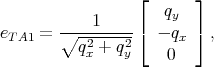 | (7.4) |
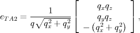 | (7.5) |
with q =  .
.
Spin relaxation rates for transitions from band i to band j by mechanism m (i.e., acoustic phonon or optical phonon), are calculated using Fermi’s second Golden Rule [107, 45, 86]
 | (7.6) |
where M is the momentum scattering (spin relaxation) matrix element, the material volume is chosen as the unit volume, 4π for spin relaxation accounts for the fact that the net number of spin polarized electrons changes by two with each spin flip [107].
The acoustic phonons scattering rate for the wave vector Ki in subband i is written as [35]
 | (7.7) |
Here, q =  is the phonon wave vector, Dαβ
 is the deformation potential, α,β = {x,y},
eβ
is the deformation potential, α,β = {x,y},
eβ = {eLA
 ,eTA1
,eTA1 ,eTA2
,eTA2 } is the polarization vector.
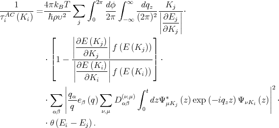
By applying Fubini’s theorem the modulus in Equation 7.7 is replaced with the repeated integral
![∫ ∫
----1---- 4-πkBT- ∑ 2π dϕ- ∞ -dqz---Kj----
τAC (K ) = ℏ ρυ2 2π (2π)2 ||∂Ej ||⋅
i i j 0 - ∞ ||----||
⌊ | | ⌋ ∂Kj
|∂E--(Kj-)|
| || ∂K ||f (E (Kj ))|
⋅|⌈1 - -|-----j--|----------|⌉ ⋅
||∂E-(Ki-)||f (E (K ))
| ∂Ki | i
∫ t∫ t[ ]
⋅ Ψ† (z)M AC ΨiKi (z ) ⋅
0 0 jKj
[ † ′ AC ′ ] ′ ′
⋅ Ψ jKj (z )M ΨiKi (z ) IAC exp(- iqz|z - z |)dzdz ⋅
⋅ θ(E - E ).
i j](disser189x.png) | (7.8) |
where MAC is the deformation potential matrix, the exact form of the matrix depends on phonon mode and is given further,
the  AC term depends on the spin-flip process and the phonon mode [107, 106]. By replacing the order of the integration
in Equation 7.8 the acoustic phonon relaxation rate is written as
AC term depends on the spin-flip process and the phonon mode [107, 106]. By replacing the order of the integration
in Equation 7.8 the acoustic phonon relaxation rate is written as
![⌊ ||∂E (K )|| ⌋
∑ ∫ 2π ||------j-||f (E (Kj))
---1-----= 4πkBT-- dϕ---1--|-Kj--|||1 - |--∂Kj---|----------|| ⋅
τAiC (Ki) ℏρ υ2 0 2π (2π)2|∂Ej--|⌈ |∂E-(Ki-)| ⌉
j ||∂K || || ∂K ||f (E (Ki))
∫ t∫ t[ j] [ i ]
† AC † ′ AC ′
⋅ 0 0 Ψ jKj (z) M ΨiKi (z) ΨjKj (z) M ΨiKi (z ) ⋅
∫ ∞
⋅ IAC exp (- iqz|z - z′|) dqzdzdz′⋅
-∞
⋅ θ(Ei - Ej) .](disser190x.png) | (7.9) |
Intervalley g-Process Spin Relaxation.
The g-process describes scattering between opposite valleys. Following [107, 106] the AC ≡ 1 for intervalley scattering.
By taking into account the Dirac delta function
 | (7.10) |
and applying the following property of the Dirac delta function
![∫ [ ]
dz′ Ψ † (z′)M AC Ψ (z′) δ(z - z′) = Ψ † (z) M AC Ψ (z) ,
jKj iKi jKj iKi](disser192x.png) | (7.11) |
Equation 7.9 is simplified to [87]
![⌊ | | ⌋
∫ ||∂E-(Kj-)||f (E (K ))
1 4πkBT ∑ 2π dϕ 1 Kj | | ∂Kj | j |
-LA------= ----2-- -------2||-----|||⌈1 - ||--------||----------|⌉ ⋅
τi (Ki) ℏ ρυLA j 0 2π (2π) |∂Ej--| |∂E-(Ki-)|f (E (Ki))
|∂Kj | | ∂Ki |
∫ t[ ][ ]
⋅ 2 π Ψ†jKj (z)M AC ΨiKi (z) Ψ †jKj (z) M ACΨiKi (z) dz⋅
0
⋅ θ (Ei - Ej) ,](disser193x.png) | (7.12) |
where υLA = 8700 [51], the matrix MAC (for the intervalley g-process spin relaxation denote it by M′) contains the Elliott
and Yafet contributions [107] is written as
[51], the matrix MAC (for the intervalley g-process spin relaxation denote it by M′) contains the Elliott
and Yafet contributions [107] is written as
![[ ]
′ MZZ MSO
M = M †SO MZZ ,](disser195x.png) | (7.13) |
![[ ]
Ξ 0
MZZ = 0 Ξ ,](disser196x.png) | (7.14) |
![[ ]
0 DSO (ry - irx)
MSO = DSO (- ry - irx) 0 ,](disser197x.png) | (7.15) |
where Ξ = 12eV is the acoustic deformation potential,  = Ki + Kj, and DSO = 15meV/k0 [107] with
k0 = 0.15 ⋅ 2π∕a which is defined as the position of the valley minimum relative to the X-point in unstrained
silicon.
= Ki + Kj, and DSO = 15meV/k0 [107] with
k0 = 0.15 ⋅ 2π∕a which is defined as the position of the valley minimum relative to the X-point in unstrained
silicon.
Intravalley Transversal Acoustic Phonons Spin Relaxation.
Intrasubband transitions are important for the contributions determined by the shear deformation potential. The AC
due to the transversal acoustic phonons is [106]
 | (7.16) |
Applying the theory of residues with Q2 = q x2 + q y2, the following integral is calculated
![∫ ′ ∫ ′
∞ q2ze--iqz|z-z-| ∞ -----q2ze-iqz|z-z|-----
(Q2 + q2)2 dqz = (iQ - q )2 (iQ + q )2 dqz =
-∞ z -∞ [( z z)| ]
d q2ze-iqz|z- z′| |
= - 2πi -------------2- || =
dqz (iQ - qz) qz=-iQ
π1 - Q |z - z′| -Q |z-z′|
= --------------e .
2 Q](disser200x.png) | (7.17) |
The matrix MAC for the intrasubband transversal acoustic phonons (M) is written as
 | (7.18) |
Here D=14eV is the shear deformation potential.
Then Equation 7.9 for the intrasubband transversal acoustic phonons is then written as
![⌊ || || ⌋
∫ |∂E-(Kj-)|f (E (Kj))
----1---- 4πkBT--∑ 2π 1----1-----|Kj-|-- || |-∂Kj----|----------||
τTA (Ki) = ℏ ρυ2 2π (2π)2||∂E (Kj) ||⌈1 - ||∂E (Ki )|| ⌉ ⋅
i TA j 0 ||-------- || ||--------||f (E (Ki))
∫ ∫ ∂Kj ∂Ki
t t ( ∘ --2---2 ′)
⋅ exp - qx + qy |z - z | ⋅
0[ 0 ]† [ ]
⋅ π- Ψ † (z)M Ψ (z) Ψ† (z′)M Ψ (z′) ⋅
2[ jKj- σ iKiσ j]Kj- σ iKiσ
4q2q2 (1 - |z - z′|∘q2--+-q2)
⋅ --x-y---(∘--------)3-x----y- dzdz′dφ
q2x + q2y](disser202x.png) | (7.19) |
where ρ=2329 is the silicon density [51], υTA=5300
 is the transversal phonons’ velocity,
  = Ki - Kj.
Intravalley Longitudinal Acoustic Phonon Spin Relaxation.
The AC due to the longitudinal acoustic phonon is given by [106]
 | (7.20) |
Applying theory of residues with Q2 = q x2 + q y2, the following integral is calculated
![∫ ∞ -iqz|z-z′| ∫ ∞ -iqz|z- z′|
-e--------dq = ------e-------------dq =
- ∞ (Q2 + q2z)2 z -∞ (iQ - qz)2(iQ + qz)2 z
[ ( -iq |z- z′|) | ]
-d-- -e--z----- ||
= - 2πi dqz (iQ - qz)2 | =
qz=- iQ
πQ-|z --z′|-+-1 -Q |z-z′|
= 2 Q3 e .](disser207x.png) | (7.21) |
The matrix MAC for the intrasubband longitudinal acoustic phonons is the same as in Equation 7.18.
From this follows, the intravalley spin relaxation rate due to longitudinal acoustic phonons is calculated as [87]
![∫ 2π
----1---- 4-πkBT- ∑ -1---1---|--|Kj-|--|
τLiA (Ki ) = ℏρυ2LA 0 2π (2π)2 |∂E (Kj )|⋅
j ||--------||
⌊ | | ⌋∂Kj
||∂E--(Kj)||
| | ∂Kj | f (E (Kj ))|
⋅|⌈1 - ||--------||-----------|⌉ ⋅
|∂E--(Ki)| f (E (Ki ))
| ∂Ki |
∫ t∫ t ( ∘ ------- )
⋅ exp - q2x + q2y |z - z′| ⋅
[0 0 ] [ ]
† * † ′ ′
⋅ ΨjKj-σ (z)M ΨiKiσ (z) ΨjKj- σ (z )M ΨiKiσ (z) ⋅
π 4q2q2 [∘ ------- ]
⋅-(∘----x-y-)3- q2x + q2y |z - z′| + 1 dzdz′dφ.
2 q2x + q2y](disser208x.png) | (7.22) |
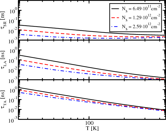
The dependence of the spin lifetime on temperature for phonon scattering, and surface roughness scattering for different carrier concentrations is shown in Figure 7.9. The spin relaxation is more efficient for higher carrier concentrations for all three considered mechanisms. While the temperature increases, the difference between the spin lifetimes for different values of the electron concentration becomes less pronounced. Figure 7.9 also shows that the surface roughness mechanism dominates for all concentration values. Spin relaxation due to transversal acoustic phonons is the weakest among the three considered mechanisms.
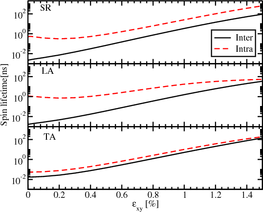
Figure 7.10 demonstrates that the main contribution to spin relaxation comes from the intersubband processes due to the presence of the spin hot spots characterized by the sharp peaks of the intersubband spin relaxation matrix elements. Their position is shown in Figure 7.11. For higher shear strain values the hot spots are pushed to higher energies, away from the subband minima (inset in Figure 7.11). This results in a strong increase of the spin lifetime with shear strain for surface roughness and the phonon mechanisms as shown in Figure 7.12.
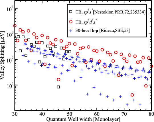
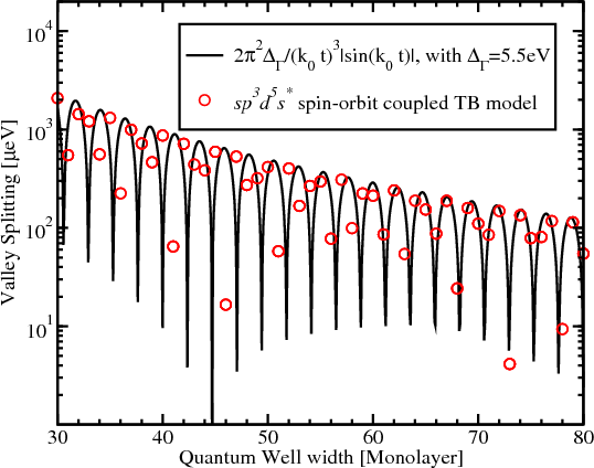
The [001] equivalent valley coupling through the Γ-point results in a subband splitting in confined electron structures [5]. The values of the valley splitting obtained from a 30-band k⋅p model [97], an atomistic tight-binding model [82], and sp3d5s* code are shown in Figure 7.13. Although looking irregular, the results follow a certain law. Figure 7.14 demonstrates a good agreement of the results of the tight-binding calculations with the analytical expression for the subband splitting [111]
 | (7.23) |
where ΔΓ is the splitting at Γ point,k0Γ = 0.85 , a is the lattice constant, and t is the film thickness. The good agreement is
found for the value ΔΓ=5.5eV.
, a is the lattice constant, and t is the film thickness. The good agreement is
found for the value ΔΓ=5.5eV.
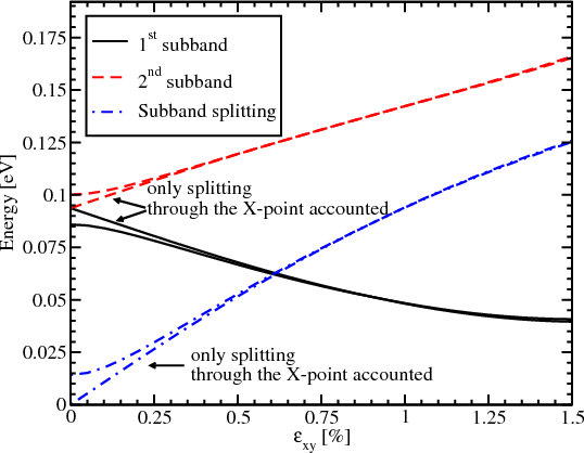
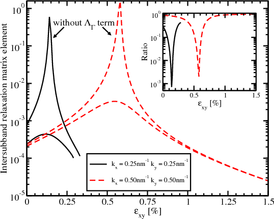
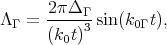
Figure 7.15 shows the dependence of the lowest unprimed subbands energies and their splitting on shear strain with and without accounting for the ΛΓ term. The unprimed subbands are degenerate at zero strain without the ΛΓ term. The ΛΓ term lifts the degeneracy while shear strain gives the major contribution to the splitting at high strain values. The surface roughness scattering matrix elements are taken to be proportional to the square of the product of the subband wave function derivatives at the interface [35]. The electron-phonon scattering is accounted for by the deformation potential approximation [87]. The surface roughness intersubband spin relaxation matrix elements with and without the ΔΓ term are shown in Figure 7.16. The difference in the matrix elements’ values calculated with and without the ΔΓ term (inset Figure 7.16) can reach two orders of magnitude. Hence, the valley coupling through the Γ-point must be taken into account for the accurate spin lifetime calculations.
The hot-spot peaks shown in Figure 7.11 becomes smoother if the Γ-point splitting is considered (Figure 7.18). However, the peaks are still well-pronounced and follow the same trend.
The peaks on the matrix elements’ dependences (Figure 7.16) are correlated with the unprimed subband splitting minima (Figure 7.17). For higher strain values the peaks corresponding to strong spin relaxation hot spots are pushed towards unoccupied states at higher energies (Figure 7.17). This leads to the strong increase of the spin lifetime demonstrated in Figure 7.19. The increase is less pronounced, if the ΛΓ term responsible for the valley splitting in relaxed films is taken into account. However, even in this case the spin lifetime is boosted by almost two orders of magnitude.
The primed subbands are governed by the following Hamiltonian [111]
![[ ]
′ H ′1 H ′3
H = H ′3 H ′2 ,](disser222x.png) | (7.24) |
where H1′, H 2′, and H 3′ are written as
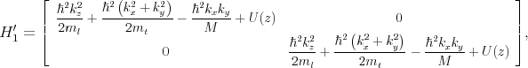 | (7.25) |
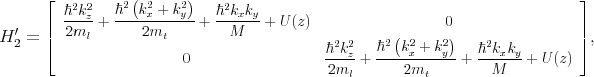 | (7.26) |
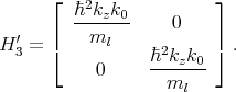 | (7.27) |
A quantization along X-axis is assumed.
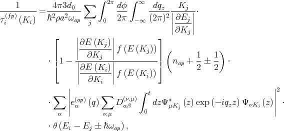
The f-process describes scattering between valleys that reside on perpendicular axes. The spin relaxation is calculated by [35]
 | (7.28) |
a defines the silicon lattice constant, d0 is the optical deformation potential, ωop denotes the frequency of the optical phonons, and nop describes the Bose occupation factor
 | (7.29) |
The relaxation rate for the transition between primed and unprimed subbands is given by [35]
 | (7.30) |
ρj(E) is the density of states for subband j and MOP is written as
 | (7.31) |
with Dop = 6.5meV [107].
In Figure 7.20 and Figure 7.21 the dispersion of the first primed subband in films with thicknesses of 2.1nm and 5nm, respectively, is compared. The minimum energy of the subband is located at the point kz = k0, ky = 0, and its value for an infinite potential square well is determined by
 | (7.32) |
The values of the subband minima for the well thickness of 2.1nm and 5nm are 0.44eV and 0.08eV, respectively. These values are in good agreement with Figure 7.20 and Figure 7.21.
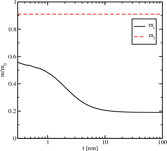
The dependence of the longitudinal and transversal effective masses on the well thickness is shown in Figure 7.22. The longitudinal effective mass ml = 0.91m0 does not depend on the thickness. In sharp contrast, the effective mass mt shows a strong increase as the film thickness reduces, in agreement with earlier predictions [111].
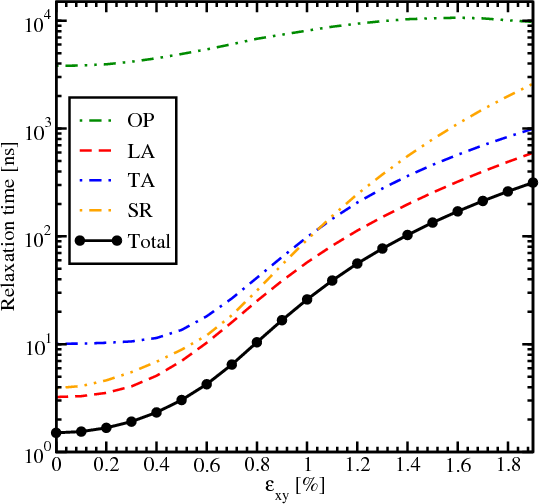
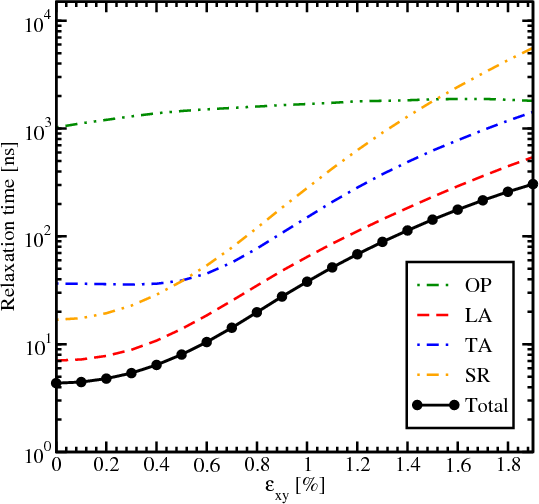
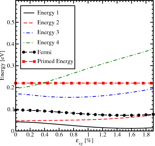
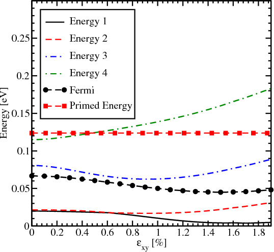
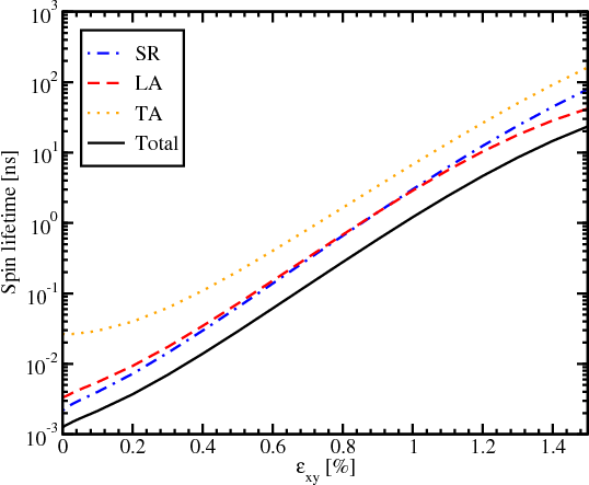
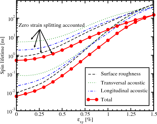
Figure 7.23 and Figure 7.24 show the total spin lifetime and contributions due to acoustic, optical phonons, and surface roughness as a function of strain for two different thicknesses (3nm and 4nm). For the film of 3nm thickness the contribution due to longitudinal acoustic phonons (LA) is close to the contribution from surface roughness for small shear strain values. Further increase of strain makes LA phonons the main contributors to the total spin lifetime. For the thicker film shown in Figure 7.24 the total spin lifetime mainly follows the same trend as the longitudinal acoustic phonons spin relaxation. Interestingly, the intersubband optical phonons calculated as g-process can be safely ignored for the film of 3nm thickness, while their contribution for the film of 4nm thickness is more considerable. The dependence of g-process phonons on strain is not so significant as the surface roughness, intrasubband scattering, and f-process scattering. Thus, for thicker films the effect of several orders of magnitude increase of spin lifetime in strained films should not be observed.
The dependence of energies for primed and unprimed subbands on strain for kx = 0 and ky = 0 together with the Fermi energy is shown in Figure 7.25 and Figure 7.26 for 3nm and 4nm, respectively. Energy 1 and Energy 2 stand for the lowest subbands of the two opposite valleys along [001] direction. Energy 3 and Energy 4 stand for the second unprimed subbands. The increasing importance of the g-process shown in Figure 7.24 compared to Figure 7.23 comes from the fact that the distance between the Fermi energy and the lowest energy in the primed subband decreases with thickness increasing. The occupation of the second subband become less pronounced at high strain as is confirmed by the Fermi level dependence for both thickness values (Figure 7.25 and Figure 7.26).