3.2.1 Mathematical Background

Response Surface Methodology [6] is a technique used to create mathematical models for the relationship between one or more responses and a set of input variables. The most widely used model functions are polynomials of the second order,

$$\hat y(x_1,\dots,x_n) = a_0 + \sum_{i=1}^{n} a_i x_i + \sum_{i=1}^{n} \sum_{j=i}^{n} a_{ij} x_i x_j$$ (3.1)

where n denotes the number of input parameters. The data from the experiment data is used to validate the response surface. If the number of experimental points is m the vector $\vec{y}$ (with the dimension m) represents the results of the experiments.

The results of the experiments $\vec{y} \in \mathbb{R}^{m}$ can be written in the vector

$$\vec{y} = \left ( \begin{array}{c} y{\{1\}} \\ \vdots \\ y{\{m\}} \\ \end{array} \right )$$ (3.2)

with the dimension m, where the variable $y{\{m\}}$ represents the response value of the m-th evaluation.

The model function can be represented by the matrix $\mathcal{Z} \in \mathbb{R}^{m \times k}$ which consists of the multiplied values of the input parameters. An example of a quadratic model function is this matrix

$$\mathcal{Z} = \left ( \begin{array}{ccccccc} 1 & x_1{\{... ...}} & \cdots & x_n{\{m\}}x_n{\{m\}} \\ \end{array} \right ) .$$ (3.3)

Each column of matrix $\mathcal{Z}$ is built from the parameter values of an experimental point. The number of the experimental points m must be equal or greater than the dimension of the vector $\vec{a}$ (k).

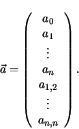
The unknown parameter vector of the model function which is expressed by

$$\vec{a} = \left ( \begin{array}{c} a_0 \\ a_1 \\ \vdots \\ a_n \\ a_{1,2} \\ \vdots \\ a_{n,n} \end{array} \right ) .$$ (3.4)

Using these matrixes and vectors, (3.1) for all experimental points of the experiment table can be written as

$$\vec{\hat y} = \mathcal{Z} \vec{a} .$$ (3.5)

In general it is not possible to find a vector $\vec{a}$ where all data points match exactly the polynomial function defined by (3.1). An error $\vec{\epsilon}$ between the real values, resulting from measurement or simulation, and the values calculated from the response surface can be calculated by

$$\vec{y} = \vec{\hat y} + \vec{\epsilon} = \mathcal{Z} \vec{a} + \vec{\epsilon} .$$ (3.6)