A. First and Second Quantization

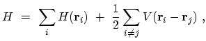
In condensed matter physics one is typically concerned with calculating physical observables from a microscopic description of the system under consideration. Such microscopic models are usually defined by the system HAMILTONian $H$. In many cases of interest the HAMILTONian takes the form

$$\displaystyle H \ = \ \sum_{i}H({\bf r}_{i})\ + \ \frac{1}{2}\sum_{i\neq j} V({\bf r}_i-{\bf r}_j) \ ,$$ (A.1)

where the first term contains a summation of single-particle HAMILTONians and $V$ is the interaction potential between particles. The quantity ${\bf r}_{i}$ denotes the coordinate of the $i\mathrm{th}$ particle, including any discrete variables such as spin for a system of FERMIons. The summation of single-particle HAMILTONians by itself is just as simple to solve as each HAMILTONian alone. One solves the dynamics of one particle, and the total properties are the summation of the individual ones. The term which makes the HAMILTONian hard to solve is the particle-particle interaction $V({\bf r}_i-{\bf r}_j)$. This term is multiplied by one-half since the double summation over $(ij)$ counts each pair twice.

Together with an appropriate number of boundary conditions the basic problem is the solution of the many-particle SCHRÖDINGER equation

$$\displaystyle i\hbar \partial_t \Psi({\bf r}_1,{\bf r}_2,\ldots,{\bf r}_N,t) \ = \ H \Psi({\bf r}_1,{\bf r}_2,\ldots,{\bf r}_N,t)\ ,$$ (A.2)

where $\Psi({\bf r}_1,{\bf r}_2,\ldots,{\bf r}_N,t)$ is the many-particle wave function that in principle contains all relevant information about the state of the system. One can start by expanding the many-particle wave function $\Psi$ in a complete set of symmetrized or anti-symmetrized products of time-independent single-particle wave functions for Bosons or FERMIons, respectively [189]. In principle, the $N$-body wave function contains all information, but a direct solution of the SCHRÖDINGER equation is impractical. Therefore, it is necessary to apply other techniques, and we shall rely on second quantization, quantum field theory, and the use of GREEN's functions.

Historically, quantum physics first dealt only with the quantization of the motion of particles, leaving the electromagnetic field classical (SCHRÖDINGER, HEISENBERG, and DIRAC, 1925-26). Later also the electromagnetic field was quantized (DIRAC, 1927), and even the particles themselves got represented by quantized fields (JORDAN and WIGNER, 1927), resulting in the development of quantum electrodynamics and quantum field theory in general.

By convention, the original form of quantum mechanics is denoted first quantization, while quantum field theory is formulated in the language of second quantization. Second quantization greatly simplifies the discussion of many interacting particles. This approach merely reformulates the original SCHRÖDINGER equation. Nevertheless, it has the advantage that in second quantization operators incorporate the statistics, which contrasts with the more cumbersome approach of using symmetrized or anti-symmetrized products of single-particle wave functions.

In the second quantization formalism a quantum mechanical basis is used that describes the number of particles occupying each state in a complete set of single-particle states. For this purpose the time-independent abstract state vectors for an $N$-particle system are introduced

$$\vert n_{1},n_{2},\ldots\rangle\ ,\ \mathrm{where}\ \sum_{j}n_{j}\ = \ N \ .$$ (A.3)

The notation means that there are $n_{1}$ particles in the state $1$, $n_{2}$ particles in the state $2$, and so forth. It is therefore natural to define occupation number operators $\hat{n}_{j}$ which have the basis states $\vert n_{j}\rangle$ as eigenstates, and have the number $n_{j}$ of particles occupying the state $j$ as eigenvalues $\hat{n}_{j}\vert n_{j}\rangle=n_{j}\vert n_{j}\rangle$. For FERMIons $n_{j}$ can be 0 or $1$, while for Bosons it can be any non-negative number.

To connect first and second quantization, annihilation and creation operators $c$ and $c^\dagger$ for FERMIons and $b$ and $b^\dagger$ for Bosons are introduced. These operators satisfy either the commutation^A.1 or anti-commutation^A.2 rules

$$\begin{array}{ll} [c_{i},c_{j}]_{+} \ = \ 0\ , \hspace*{40pt}... ...{40pt} [b_{i}^\dagger,b_{j}^\dagger]_{-} \ = \ 0\ . \end{array}$$ (A.4)

All of the properties of these operators follow directly from the commutation or anti-commutation rules. The annihilation operators, $c_{i}$ and $b_{i}$, decrease the occupation number of the state $i$ by 1, whereas the creation operators, $c_{i}^{\dagger}$ and $b_{i}^{\dagger}$, increase the occupation number of the state $i$ by 1.

The HAMILTONian in (A.1) can be written in terms of annihilation and creation operators

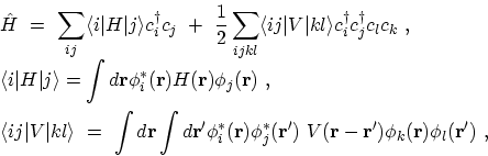$$\begin{array}{l} \displaystyle \hat{H}\ = \ \sum_{ij} \langle... ...}) {\phi}_{k}({\bf {r}}) {\phi}_{l}({\bf {r'}}) \ , \end{array}$$ (A.5)

where $\phi_{i}({\bf {r}})$ are the single-particle wave functions and the circumflex denotes an operator in the abstract occupation-number Hilbert space. In this form, the matrix elements of the single-particle HAMILTONian and the interaction potential taken between the single-particle eigenstates of the SCHRÖDINGER equation in first quantization are merely complex numbers multiplying operators.

It is often convenient to form a linear combination of the annihilation and creation operators

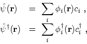$$\begin{array}{ll} \displaystyle \hat{\psi}({\bf {r}}) \ &\dis... ...um_{i} \phi_{i}^\dagger({\bf {r}}) c_{i}^\dagger\ , \end{array}$$ (A.6)

where the sum is over the complete set of single-particle quantum numbers. The so-called field operators $\hat{\psi}({\bf {r}})$ and $\hat{\psi}^\dagger({\bf {r}})$ satisfy simple commutation or anti-commutation relations

$$\begin{array}{lll} \displaystyle [\hat{\psi}({\bf {r}}),\hat{... ...,\hat{\psi}^\dagger({\bf {r'}})]_{\pm} \ & = \ 0\ , \end{array}$$ (A.7)

where the plus (minus) sign refers to FERMIons (Bosons). The field operator $\hat{\psi}({\bf {r}})$ annihilates and $\hat{\psi}^{\dagger}({\bf {r}})$ creates a particle at place ${\bf {r}}$. The HAMILTONian operator can be rewritten in terms of these field operators as follows

$$\displaystyle \hat{H} \ = \ \int d{\bf {r}} \hat{\psi}^\dagger({\... ... {r'}}) V({\bf {r}}-{\bf {r'}}) \hat{\psi}({\bf {r'}}) \hat{\psi}({\bf {r}})\ .$$ (A.8)

In this form, the HAMILTONian suggests the name second quantization, since the above expression looks like the expectation value of the HAMILTON ian taken between wave functions. Both (A.5) and (A.8) are equivalent since the integration over spatial coordinates produces the single-particle matrix elements of the kinetic energy, potential and interaction potential energy, leaving a sum of these matrix elements multiplied by the appropriate annihilation and creation operators.

The methods of quantum field theory also allow us to concentrate on the few matrix elements of interest, thus avoiding the need for dealing directly with the many-particle wave function and the coordinates of all the remaining particles. Finally, the GREEN's functions contain the most important physical information such as the ground-state energy and other thermodynamic functions, the energy and life time of excited states, and the response to external perturbations. Unfortunately, the exact GREEN's functions are not easier to determine than the original wave function, and we therefore make use of perturbation theory which can be expressed in the systematic language of FEYNMAN  rules and diagrams. These rules allow one to evaluate physical quantities to any perturbation order.

M. Pourfath: Numerical Study of Quantum Transport in Carbon Nanotube-Based Transistors