B.5 Imaginary Time Operators
At finite temperature under thermodynamic equilibrium the state of a system is
described by the equilibrium density operator
 . For a given
the ensemble average of any operator
. For a given
the ensemble average of any operator  can be calculated as
(see (3.11))
can be calculated as
(see (3.11))
![\begin{displaymath}\begin{array}{ll}\displaystyle \langle \hat{O}\rangle \ &\dis...
...{K}} \hat{O}]} {\mathrm{Tr}[e^{-\beta\hat{K}}]} \ , \end{array}\end{displaymath}](img1118.png) |
(B.25) |
where
 may be interpreted as a grand
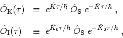
canonical HAMILTONian. For any SCHRÖDINGER operator
may be interpreted as a grand
canonical HAMILTONian. For any SCHRÖDINGER operator
 , the
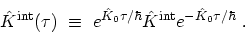
so called modified HEISENBERG and interaction pictures can be introduced as
, the
so called modified HEISENBERG and interaction pictures can be introduced as
 |
(B.26) |
where  includes only the non-interacting part of
  . It
should be noticed that
. It
should be noticed that
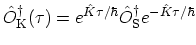 is not
the adjoint of
is not
the adjoint of
 as long as
  is real. If
is interpreted as a complex variable, however, it may be analytically continued
to a pure imaginary value
is real. If
is interpreted as a complex variable, however, it may be analytically continued
to a pure imaginary value  . The resulting expression
 then becomes the true adjoint of
and is formally identical with the original
HEISENBERG picture defined in (B.12), apart from
the substitution of for
then becomes the true adjoint of
and is formally identical with the original
HEISENBERG picture defined in (B.12), apart from
the substitution of for  . For this reason
(B.26) are sometimes called imaginary-time operators.
. For this reason
(B.26) are sometimes called imaginary-time operators.
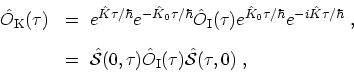
The modified HEISENBERG and interaction pictures are related by (compare
(B.13) and
(B.14))
 |
(B.27) |
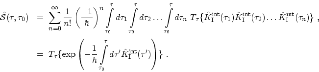
where the operator
 is defined by (compare (B.17))
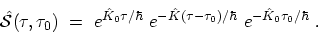 |
(B.28) |
Note that
is not unitary, but it still
satisfies the group property
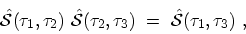 |
(B.29) |
and the boundary condition
 |
(B.30) |
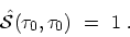
In addition, the equation of motion of
is calculated as
 |
(B.31) |
where
 |
(B.32) |
It follows that the operator
obeys essentially the same
differential equation as the unitary operator introduced in (B.15), and one
may immediately write down the solution (compare (B.24))
 |
(B.33) |
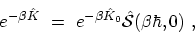
If is set equal to
 , (B.28) may be rewritten as
 |
(B.34) |
which relates the many particle density operator to the single-particle
density operator by means of an imaginary time-evolution operator.
M. Pourfath: Numerical Study of Quantum Transport in Carbon Nanotube-Based Transistors