3.3.2 Contour-Ordered GREEN's Function

To express the field operators in the interaction representation an operator $\hat{S}$ is defined (see Appendix B.4) and applied for calculating the GREEN's functions as in Section 3.1.1. The time in (3.8) is taken over the interval $(-\infty,\infty)$. The state at $t \rightarrow -\infty$ is well defined as the ground-state of the non-interacting system $\vert\phi_{0}\rangle$. The interactions are turned on slowly. At $t=0$ the fully interacting ground state is $\vert\Psi(0)\rangle = \hat{S}(0,-\infty)\vert\phi_{0}\rangle$. The state at $t\rightarrow\infty$ must be defined carefully. If the interactions remain on, then this state is not well described by the non-interacting ground state. Alternatively, one could require that the interactions are turned off at large times, which returns the system to the ground-state $\vert\phi_{0}\rangle$.

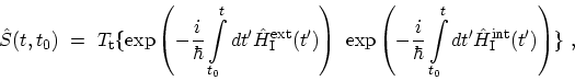
SCHWINGER [92] suggested another method of handling the asymptotic limit $t \rightarrow -\infty$. He proposed that the time integral in the $\hat{S}$ operator has two parts; one goes from $(-\infty,t)$ while the second goes from $(t,-\infty)$. The integration path is a contour, which starts and ends at $-\infty$. The advantage of this method is that one starts and ends the $S$ operator expansion with a known state $\vert\Psi(-\infty)\rangle=\vert\phi_{0}\rangle$. Instead of the time-ordering operator (B.21), a contour-ordering operator can be employed. The contour-ordering operator $T_\mathrm{C}$ orders the time labels according to their order on the contour ${C}$. Under equilibrium condition the contour-ordered method gives results that are identical to the time-ordered method described in Section 3.1.1. The main advantage of the contour-ordered method is in describing non-equilibrium phenomena using GREEN's functions. Non-equilibrium theory is entirely based upon this formalism, or equivalent methods.

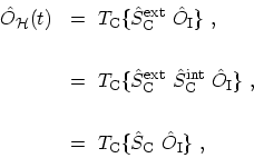
Any operator $\hat{O}_\mathcal{H}$ in the HEISENBERG picture can be transformed into the interaction picture (see (B.13))

$$\begin{array}{l}\displaystyle \hat{O}_\mathcal{H} \ = \ \hat{S}(t_0,t)\ \hat{O}_\mathrm{I}\ \hat{S}(t,t_0)\ . \end{array}$$ (3.19)

Analogous to the derivation of (B.24), it can be shown that the $\hat{S}$ operator is given by

$$\begin{array}{l} \displaystyle \hat{S}(t,t_{0}) \ = \ T_\math... ...t{H}^\mathrm{int}_\mathrm{I}(t')}\right) \} \ , \end{array}$$ (3.20)

where the operators are in the interaction representation. The ordinary time-ordering can also be written as ordering along contour branches ${C}_1$ and ${C}_2$ as depicted in Fig. 3.1

$$\begin{array}{l}\displaystyle \hat{S}(t,t_0) \ \displaystyle... ... \hat{H}^\mathrm{int}_\mathrm{I}(t)}\right)\} \ . \end{array}$$ (3.21)

By combining two contour branches, ${C}={C}_1\cup {C}_2$, (3.19) can be rewritten as

$$\begin{array}{ll}\displaystyle \hat{O}_\mathcal{H}(t) \ &\di... ...{C}\{\hat{S}_\mathrm{C}\ \hat{O}_\mathrm{I}\} \ , \end{array}$$ (3.22)

where,

$$\begin{array}{ll} \hat{S}_\mathrm{C}\ &\displaystyle = \ \ex... ...xt}_\mathrm{C}\ \hat{S}^\mathrm{int}_\mathrm{C}\ . \end{array}$$ (3.23)

Figure 3.1: The contour ${C}={C_1}\cup {C_2}$ runs on the real axis, but for clarity its two branches $C_1$ and $C_2$ are shown slightly away from the real axis. The contour ${C_i}$ runs from $t_0$ to $t_0-i\beta$.

In equation (3.17) $\hat{\rho}$ describes the equilibrium state of the system before the external perturbation $\hat{H}^\mathrm{ext}$ is turned on. Interactions $\hat{H}^\mathrm{int}$, which are switched on adiabatically at $-\infty$, are present in $\hat{\rho}$. However, to apply WICK's theorem (Section 3.4.1), one has to work with non-interacting operators. A methodology similar to the MATSUBARA theory can be applied to express the many-particle density operator $\hat{\rho}$ in terms of the single-particle density operator $\hat{\rho}_0$, see Appendix B.5. If the contour ${C_i}=[t_0,t_0-i\beta]$ is chosen (Fig. 3.1), then (B.34) takes the form

$$\begin{array}{l}\displaystyle e^{-\beta \hat{K}} \displaystyle = \ e^{-\beta \hat{K}_0} \ {\hat{S}}_{C_i} \ . \end{array}$$ (3.24)

Therefore, (3.17) can be rewritten as

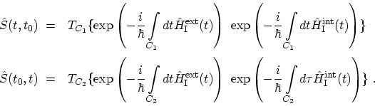
$$\langle \hat{O}_\mathscr{H}(t) \rangle \ = \frac{\mathrm{Tr}[e^{-... ...}_\mathscr{H}(t) ]} {\mathrm{Tr}[e^{-\beta \hat{K}_0}T_{C_i}\hat{S}_{C_i}]}\ ,$$ (3.25)

Using the relations (3.22) and (3.25), the GREEN's function in (3.18) becomes [196]

$$\begin{array}{l}\displaystyle G({\bf {r}},t,{\bf {r'}},t') \... ...}_0}T_{C_i} \hat{S}_{C_i}\ T_{C} \hat{S}_{C}]} \ . \end{array}$$ (3.26)

The twofold expansion of the density operator and the field operators may conveniently be combined to a single expansion. The two contours ${C_i}$ and ${C}$ can be combined together, ${C^*}={C}\cup {C_i}$ (Fig. 3.2), and a contour-ordering operator $T_{C^*}=T_{C_i}T_{C}$, which orders along ${C^*}$, can be introduced. Hence, a point on ${C}$ is always earlier than a point on ${C_i}$. Furthermore, we define an interaction representation with respect to $\hat{H}_0$ on ${C}$ and with respect to $\hat{K}_0$ on ${C_i}$. Therefore, the GREEN's function in (3.18) is given by

$$\begin{array}{ll}\displaystyle G({\bf {r}},t,{\bf {r'}},t') ... ...dagger_{\mathrm{I}}({\bf {r}'},t')\} \rangle_0 \ , \end{array}$$ (3.27)

where $\langle\ldots\rangle_0$ represents the statistical average with respect to $\hat{\rho}_0$. From here we assume that all statistical averages are with respect to $\hat{\rho}_0$ and drop the 0 from the brackets $\langle\ldots\rangle_0$.

Figure 3.2: The contour ${C^*}={C_i}\cup {C}$, runs from $t_0$ to $t_0$ and from $t_0$ to $t_0-i\beta$.

M. Pourfath: Numerical Study of Quantum Transport in Carbon Nanotube-Based Transistors