3.8.1 The KADANOFF-BAYM Formulation
The starting point of the derivation is the differential form of the
DYSON equation. By assuming that
![$ [i\hbar\partial_{t_1}-\hat{H}_0(1)]G_0(12)=\delta_{1,2}$](img646.png) ,
equation (3.44) and (3.45) can be rewritten as [203]
,
equation (3.44) and (3.45) can be rewritten as [203]
 |
(3.60) |
 |
(3.61) |
Note that the singular part of the self-energy on the contour, which
corresponds to the HARTREE self-energy (Section 3.6), does not
appear explicitly in the kinetic equations, but is included in the potential
energy of the single-particle HAMILTONian  , see (F.7).
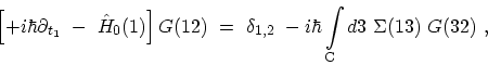
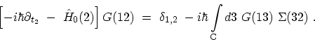
Using the LANGRETH rules (Table 3.1) and fixing the time
arguments of the GREEN's functions in (3.60)
and (3.61) at opposite sides of the contour, one
obtains the KADANOFF-BAYM equations [93,203]
 |
(3.62) |
 |
(3.63) |
One should note that the delta-function term in (3.60) and
(3.61) vanishes identically, because the time-labels required
in the construction of  and
and  are, by the definition on different
branches of the contour.
are, by the definition on different
branches of the contour.
The KADANOFF-BAYM equations determine the time evolution of the GREEN's
functions, but they do not determine the consistent initial values. This
information is contained in the original DYSON equations
(3.44) and (3.45), and lost in the
derivation. To have a closed set of equations, the
KADANOFF-BAYM equations must be supplemented with DYSON equations for
 and
and
 . By subtracting (3.63)
from (3.62), one finds the equation satisfied by
[203]
. By subtracting (3.63)
from (3.62), one finds the equation satisfied by
[203]
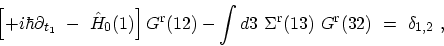 |
(3.64) |
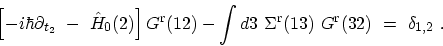 |
(3.65) |
Similar relations hold for the advanced GREEN's functions.
M. Pourfath: Numerical Study of Quantum Transport in Carbon Nanotube-Based Transistors