|
|
|
|
Previous: 4.1 Electrostatic Potential and the POISSON Equation Up: 4.1 Electrostatic Potential and the POISSON Equation Next: 4.1.2 Boundary Conditions |
|
|
|
|
Previous: 4.1 Electrostatic Potential and the POISSON Equation Up: 4.1 Electrostatic Potential and the POISSON Equation Next: 4.1.2 Boundary Conditions |
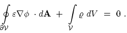 |
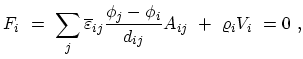
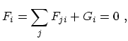
(4.3) |
![\includegraphics[width=0.3\textwidth]{figures/Box_Intg.eps}](img739.png)