4.3 Tight-Binding HAMILTONian

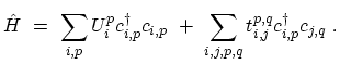
The general form of the tight-binding HAMILTONian for electrons in a CNT can be written as

$$\displaystyle \hat{H} \ = \ \sum_{i,p}U_{i}^{p}c^{\dagger}_{i,p}c_{i,p} \ + \ \sum_{i,j,p,q} t_{i,j}^{p,q}c^{\dagger}_{i,p}c_{j,q} \ .$$ (4.13)

The sum is taken over all rings $i$, $j$ along the transport direction, which is assumed to be the $z$-direction of the cylindrical coordinate system, and over all atomic locations $p$,$q$ in a ring. We use a nearest-neighbor tight-binding $\pi$-bond model [243,10]. Each atom in an $sp^{2}$-coordinated CNT has three nearest neighbors, located $a_\mathrm{C-C}$ away. The band-structure consists of $\pi$-orbitals only, with the hopping parameter $t=V_\mathrm{pp\pi}=\mathrm{-2.77~eV}$ and zero on-site potential. Furthermore, it is assumed that the electrostatic potential $U$ rigidly shifts the on-site potentials. Such a tight-binding model is adequate to model transport properties in un-deformed CNTs.

In this work we consider zigzag CNTs. However, this method can be readily extended to armchair or chiral CNTs. Within the nearest-neighbor approximation, only the following parameters are non zero [10]

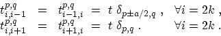$$\begin{array}{llll}\displaystyle t_{i,i-1}^{p,q}& = &t_{i-1,i... ...,i}^{p,q}\ = \ t\ \delta_{p,q}\ . &\forall i=2k \ . \end{array}$$ (4.14)

Figure 4.6 shows that a zigzag CNT is composed of rings (layers) of $A$- and $B$-type carbon atoms, where $A$ and $B$ represent the two carbon atoms in a unit cell of graphene. Each A-type ring is adjacent to a B-type ring. Within nearest-neighbor tight-binding approximation the total HAMILTONian matrix is block tri-diagonal [243]

$$\ensuremath{{\underline{H}}} = { \left[ \begin{array}{cccccc} \en... ...underline{H}}}_5 & \bullet\\ & & & & \bullet & \bullet \end{array} \right]} \ ,$$ (4.15)

where the diagonal blocks, $\ensuremath{{\underline{H}}}_i$, describe the coupling within an A-type or B-type carbon ring and off-diagonal blocks, $\ensuremath{{\underline{t}}}_1$ and $\ensuremath{{\underline{t}}}_2$, describe the coupling between adjacent rings. It should be noted that the odd numbered HAMILTONian $\ensuremath{{\underline{H}}}_i$ refer to A-type rings and the even numbered one to B-type rings. Each A-type ring couples to the next B-type ring according to $\ensuremath{{\underline{t}}}_2$ and to the previous B-type ring according to $\ensuremath{{\underline{t}}}_1$. Each B-type ring couples to the next A-type ring according to $\ensuremath{{\underline{t}}}_1$ and to the previous A-type ring according to $\ensuremath{{\underline{t}}}_2$. In a $(n,0)$ zigzag CNT, there are $n$ carbon atoms in each ring, thus, all the sub-matrices in (4.15) have a size of $n\times n$.

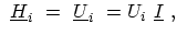
In the nearest-neighbor tight binding approximation, carbon atoms within a ring are not coupled to each other so that $\ensuremath{{\underline{H}}}_i$ is a diagonal matrix. The value of a diagonal entry is the potential at that carbon atom site. In the case of a coaxially gated CNT, the potential is constant along the CNT circumference. As a result, the sub-matrices $\ensuremath{{\underline{H}}}_i$ are given by the potential at the respective carbon ring times the identity matrix

$$\ \ensuremath{{\underline{H}}}_i \ = \ \ensuremath{{\underline{U}}}_i \ = U_i\ \ensuremath{{\underline{I}}} \ ,$$ (4.16)

Figure 4.6: Layer layout of a $(n,0)$ zigzag CNT. Circles are rings of A-type carbon atoms and squares rings of B-type carbon atoms. The coupling coefficient between nearest neighbor carbon atoms is $t$. The coupling matrices between rings are denoted by $\ensuremath{{\underline{t}}}_{1}$ and $\ensuremath{{\underline{t}}}_{2}$, where $\ensuremath{{\underline{t}}}_{1}$ is a diagonal matrix and $\ensuremath{{\underline{t}}}_{2}$ is non-diagonal.

There are two types of coupling matrices between nearest carbon rings, $\ensuremath{{\underline{t}}}_1$ and $\ensuremath{{\underline{t}}}_2$. As shown in Fig. 4.6, the first type, $\ensuremath{{\underline{t}}}_1$, only couples an A(B) carbon atom to its B(A) counterpart in the neighboring ring. The coupling matrix is just the tight-binding coupling parameter times an identity matrix,

$$\ensuremath{{\underline{t}}}_1 \ = \ t\ensuremath{{\underline{I}}} \ .$$ (4.17)

The second type of coupling matrix, $\ensuremath{{\underline{t}}}_2$, couples an A(B) atom to two B(A) neighbors in the adjacent ring. The coupling matrix is

$$\ensuremath{{\underline{t}}}_2\ = \ { \left[ \begin{array}{cccccc... ... & \\ \displaystyle & t & t & \\ & & \bullet & \bullet \end{array} \right]} \ .$$ (4.18)

The period of the zigzag CNT in the longitudinal direction contains four rings, $\mathrm{ABAB}$, and has a length of $3a_\mathrm{C-C}$. Therefore, the average distance between the rings is

$$\Delta z\ = \ \frac{3a_\mathrm{C-C}}{4} \ .$$ (4.19)

M. Pourfath: Numerical Study of Quantum Transport in Carbon Nanotube-Based Transistors