3.1.3 Shape Functions

Next: 3.2 Finite Boxes Up: 3.1 Finite Elements Previous: 3.1.2 Numerical Integration

3.1.3 Shape Functions

The essence of the finite element method, already stated above, is to approximate the unknown by an expression given as

$\displaystyle \bf u$ $\displaystyle \approx$ $\displaystyle \sum_{i=1}^{n}$ N_i^.a_i = $\displaystyle \bf N \cdot a$

(3.24)

where N_i are the interpolating shape functions prescribed in terms of linear independent functions and a_i are a set of unknown parameters. Under normal circumstances the variables are chosen to be identical with the values of the unknown function at the element nodes, thus making

u_i $\displaystyle \equiv$ a_i

(3.25)

Now consider to interpolate a constant function over the simulation domain. It is clear that a constant value of a_i specified at all nodes must result in a constant value of $\bf u$ which immediately implies that

$\displaystyle \sum_{i=1}^{n}$ N_i = 1

(3.26)

at all points of the domain. The so defined shape functions are referred to as standard shape functions and are the basics of most finite element programs. Several extensions to the standard shape functions exist and the reader is advised to relevant literature [Sch80].

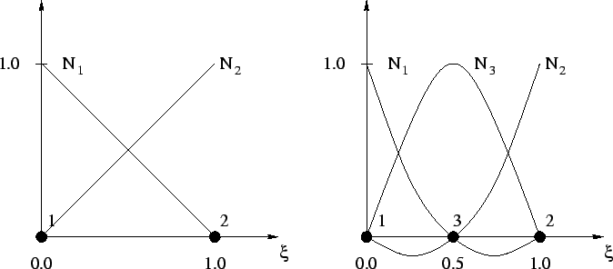
**Figure 3.3:** Linear and quadratic shape functions for one-dimensional elements
$\resizebox{15.0cm}{!}{\includegraphics{/iue/a39/users/radi/diss/fig/discrete/1Dshape.eps}}$

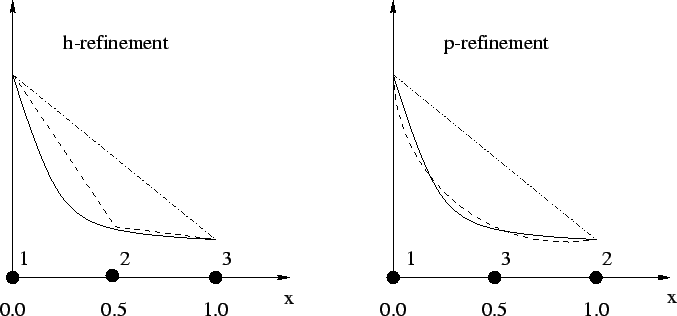
The used interpolation scheme is illustrated in Fig. 3.3 where the node points have to be multiplied with the shape functions to get the values inside the element. The order of interpolation of the shape function stipulates the accuracy of the element. Thus, there are two strategies to get high quality results (Fig. 3.4):

h-refinement: In this case the local density of elements is increased that introduces a larger number of discrete points in the areas of interest but the order of the interpolation function remains unchanged. This version is often used due to the simpler approach but especially in three dimensions the higher number of discrete points is a serious drawback.
p-refinement: Here, the order of the interpolation function is increased so that the characteristics of approximation of the element itself are better. This often reduces the amount of discrete points that are needed to represent a given function within a tolerable error level. Nevertheless, there are limits due to oscillating results in case of higher orders. Therefore shape functions up to a maximum order of three are normally used. For further increase of accuracy the h-refinement seems to be the better approach.

**Figure 3.4:** Approximation characteristics of linear and quadratic shape functions in case of h-refinement and p-refinement
$\resizebox{15.0cm}{!}{\includegraphics{/iue/a39/users/radi/diss/fig/discrete/1Dapprox.eps}}$

The shape function itself can be calculated using a polynomial approach. For linear interpolation on a one-dimensional element with two nodes a polynomial of first order

u( $\displaystyle \xi$ ) = $\displaystyle \alpha_{1}^{}$ + $\displaystyle \alpha_{2}^{}$ $\displaystyle \xi$

(3.27)

can be used. To calculate the coefficients $\alpha_{1}^{}$ and $\alpha_{2}^{}$ the values at the element nodes can be inserted into (3.27)

$\displaystyle \alpha_{1}^{}$ = u₁			(3.28)
$\displaystyle \alpha_{2}^{}$ = - u₁ + u₂			(3.29)

Substituting these results into (3.27) yields

u( $\displaystyle \xi$ ) = u₁(1 - $\displaystyle \xi$ ) + u₂ $\displaystyle \xi$ = u₁N₁( $\displaystyle \xi$ ) + u₂N₂( $\displaystyle \xi$ )

(3.30)

The same principle can be used for all other orders of interpolation as well as for different dimensions. For higher orders of interpolation derivatives are additionally used to calculate the coefficients of the polynomial.

For a summary of shape functions in one, two, and three dimensions calculated for different interpolation orders refer to Appendix B.

Next: 3.2 Finite Boxes Up: 3.1 Finite Elements Previous: 3.1.2 Numerical Integration

Mustafa Radi
1998-12-11