The Input & Control Interface is intended for the description of the complete simulation flow process within AMIGOS and includes semantics for mapping a discretized model onto a specific device structure for any complex simulation domain. It is kept as simple as possible and the syntax tries to support `language like commands'.
The user has to define which physical models and boundary conditions should be used, where to read the geometry from and which kind of grid to use for discretization. Default parameters defined in the Analytical Model Interface (AMI) can be overwritten as well as the solution methods for eventually defined derivative quantities implicitly defined. Furthermore, the order of interpolation, the time step calculation and adaptation, and the numerical solving methods (direct or iterative) are chosen within the Input & Control Interface.
AMIGOS uses an annotated mesh data structure to represent the physical structure (wafer state) of a device, including materials, interfaces, impurities, defect profiles, stresses and other characteristic quantities. The abstractions used to represent a mapping mechanism from existing models onto a given simulation domain are handled in the following sections representing the basic input needed to solve a differential equation with AMIGOS.
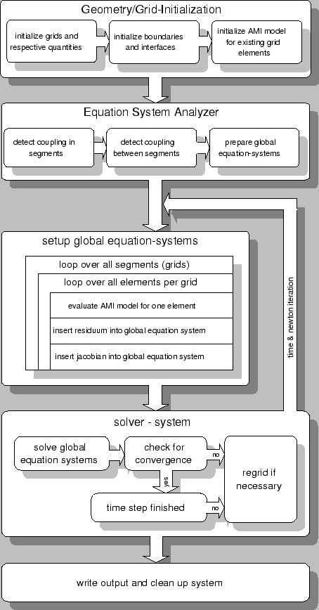
All of the remaining tasks are done automatically by the simulation system without any further user interaction. The program detects whether to use moving grids as necessary in case of, e.g., mechanical deformations as well as the dimension of the problem. It prepares all boundaries and interface grids and checks for existing interconnections between several simulation domains. All specified analytical models, all model quantities, derivatives and parameters are initialized and the necessary memory is allocated. After analyzing the partial differential equations to be solved and optimizing the defined models it prepares the global system matrices and residual vectors and starts solving. If necessary it starts a Newton iteration for nonlinear problems and adapts the grid where the error-level is greater than a given epsilon criterion. Afterwards it writes the results on a file either for later reuse or just for visualization (Fig. 4.3).